Topics Covered
On this page
- The Data Set
- Practical 1: Understanding the Data Set
- Practical 2: Data Transformations
- Practical 3: Descriptive Statistics by Scale
- Practical 4: Data Visualization
- Practical 5: Mathematical Model Building
- Practical 6: Evaluation of Model Performance
- Practical 7: Parametric Tests
- Practical 8: Non-Parametric Tests
- Writing the Statistical Report
- How Marks Are Lost
- What the Practical Record Should Contain
- Computational Statistics and R Programming, Unit 1 — the R environment, language basics, data types, import and export, missing values, subsetting, merging, the apply family and the working directory
- Unit 2 — central tendency, variability, quantiles, skewness and kurtosis, the summary functions and categorical data
- Unit 3 — histograms, boxplots, scatter plots, bar charts, residual plots and saving a plot
- Unit 4 — distributions, random sampling, \(t\) tests, \(\chi^{2}\) tests, one-way analysis of variance, \(p\) values, confidence intervals and the Wilcoxon tests
- Unit 5 — correlation, simple and multiple regression and residual diagnostics
var, the continuity correction in wilcox.test — it is named.
The Data Set
One data set carries the whole course, so that each stage can be checked against the last.
grade is derived from score and buy is the outcome the
classification analysis predicts. Every programme below begins with these lines.
customers <- data.frame(
  id     = 1:20,
  age    = c(23,45,31,58,27,39,52,34,29,48,36,41,25,55,33,44,30,50,28,38),
  income = c(40,57,37,69,36,38,63,32,35,57,42,49,26,39,48,49,23,57,27,33),
  score  = c(54,55,64,77,69,60,85,57,65,59,64,60,51,57,60,60,55,67,40,56),
  gender = factor(c("M","F","M","F","M","F","M","F","M","F",
                    "M","F","M","F","M","F","M","F","M","F")),
  buy    = c(0,1,0,1,1,0,1,0,0,1,0,0,0,0,1,1,0,1,0,0)
)
customers$grade <- cut(customers$score, breaks = c(-Inf, 57, 65, Inf),
                       labels = c("Low","Med","High"), right = FALSE)
customers$buy <- factor(customers$buy, levels = c(0,1), labels = c("No","Yes"))
Note right = FALSE. R's cut closes intervals on
the right by default, so breaks = c(-Inf, 57, 65, Inf) without it would put a
score of exactly 57 in the Low class. Boundary cases are where derived categorical
variables go wrong, and they go wrong silently.
Practical 1: Understanding the Data Set
1. Question
For the customers data, place each variable on its scale of measurement, declare the ordinal
variable so that R refuses the wrong operations, and carry out the pre-processing checks for missing values and
duplicates.
2. Aim
To identify the scale of each variable, which decides the operations that mean anything, and to check the data before any analysis.
3. Steps
- Inspect the structure, and the counts of each category.
R's class is not the scale. "numeric" covers
age(ratio) andscore(interval); "factor" coversgender(nominal) andgrade(ordinal).Scale Distinguishes Legitimate summaries Here Nominal difference only counts, mode, \(\chi^{2}\) gender,buyOrdinal difference and order median, quartiles, rank correlation, rank tests gradeInterval order and equal spacing, arbitrary zero mean, standard deviation, correlation — but not ratios score, treated as intervalRatio all of the above, plus a true zero everything, including the coefficient of variation and the geometric mean age,income - Declare grade ordinal, and see what R then allows.
Coding
grade1, 2, 3 and taking a mean produces a number, and the number is meaningless: nothing says the step from Low to Med equals the step from Med to High. Declared ordered, the median is found byquantile()and the mean is refused. - Pre-processing checks: missing values and duplicates.
The checks come in a fixed order: read and inspect; fix types; count missing values and decide (drop, impute, and by what); identify outliers without deleting them; check duplicates on the key; only then derive and transform; and split before anything is estimated if a model is to be fitted.
| Command or formula | What it does |
|---|---|
str(), sapply(d, class) | the structure and R's storage class of each column |
factor(x, levels, ordered = TRUE) | an ordinal variable: order is kept, arithmetic is refused |
colSums(is.na(d)), duplicated(key) | missing values per column; repeated keys |
4. Programme
# Practical 1: Understanding the Data Set

# The data set: twenty records
customers <- data.frame(
  id     = 1:20,
  age    = c(23,45,31,58,27,39,52,34,29,48,36,41,25,55,33,44,30,50,28,38),
  income = c(40,57,37,69,36,38,63,32,35,57,42,49,26,39,48,49,23,57,27,33),
  score  = c(54,55,64,77,69,60,85,57,65,59,64,60,51,57,60,60,55,67,40,56),
  gender = factor(c("M","F","M","F","M","F","M","F","M","F",
                    "M","F","M","F","M","F","M","F","M","F")),
  buy    = c(0,1,0,1,1,0,1,0,0,1,0,0,0,0,1,1,0,1,0,0)
)
customers$grade <- cut(customers$score, breaks = c(-Inf, 57, 65, Inf),
                       labels = c("Low","Med","High"), right = FALSE)
customers$buy <- factor(customers$buy, levels = c(0,1), labels = c("No","Yes"))

# Step 1: Inspect the structure, and the counts of each category
str(customers)
sapply(customers, class)
table(customers$grade); table(customers$gender); table(customers$buy)

# Step 2: Declare grade ordinal, and see what R then allows
customers$grade <- factor(customers$grade, levels = c("Low","Med","High"), ordered = TRUE)
quantile(customers$grade, 0.5, type = 1)   # the median of an ordered factor
mean(customers$grade)

# Step 3: Pre-processing checks: missing values and duplicates
colSums(is.na(customers))
sum(duplicated(customers$id))
sapply(customers, function(v) sum(is.na(v)))    # works for any data frame
5. Execution and Results
Step 1: Inspect the structure, and the counts of each category
'data.frame':	20 obs. of  7 variables:
 $ id    : int  1 2 3 4 5 6 7 8 9 10 ...
 $ age   : num  23 45 31 58 27 39 52 34 29 48 ...
 $ income: num  40 57 37 69 36 38 63 32 35 57 ...
 $ score : num  54 55 64 77 69 60 85 57 65 59 ...
 $ gender: Factor w/ 2 levels "F","M": 2 1 2 1 2 1 2 1 2 1 ...
 $ buy   : Factor w/ 2 levels "No","Yes": 1 2 1 2 2 1 2 1 1 2 ...
 $ grade : Factor w/ 3 levels "Low","Med","High": 1 1 2 3 3 2 3 2 3 2 ...
       id       age    income     score    gender       buy     grade
"integer" "numeric" "numeric" "numeric"  "factor"  "factor"  "factor"

 Low  Med High
   6    9    5

 F  M
10 10

 No Yes
 12   8
Step 2: Declare grade ordinal, and see what R then allows
50%
Med
Levels: Low < Med < High
[1] NA
Warning message:
In mean.default(customers$grade) :
  argument is not numeric or logical: returning NA
Step 3: Pre-processing checks: missing values and duplicates
    id    age income  score gender    buy  grade
     0      0      0      0      0      0      0
[1] 0
    id    age income  score gender    buy  grade
0 0 0 0 0 0 0 mean() of a factor is not an error in R: it returns NA and warns that the argument is not numeric or logical. The warning is the refusal; a script that ignores warnings will carry the NA on.
median() refuses a factor, even an ordered one, with the error "need numeric data". The median of an ordered factor is quantile(x, 0.5, type = 1) (types 1 and 3 are the quantile rules that pick an observed value rather than interpolate between two).
The twenty records hold two ratio variables (age, income), one interval
(score), one ordinal (grade: Low 6, Med 9, High 5) and two nominal (gender: 10 and
10; buy: No 12, Yes 8). There are no missing values and no duplicate keys. Declared ordered, grade
has median Med, and R refuses its mean — it returns NA with a warning — which is the
right answer to a meaningless question.
Practical 2: Data Transformations
1. Question
Apply standardization, min–max normalization, and the log, square-root and square transformations to
income, judging each by what it does to the skewness; and encode a cyclic variable (month) by its sine
and cosine.
2. Aim
To choose a transformation by what it does to the data, and to see why a cyclic variable needs two columns.
3. Steps
- Skewness of income under each transformation.
Judge a transformation by what it does to the skewness, not by habit.
- Standardization and normalization, written out and checked.
zuses R'ssd, which divides by \(n-1\);scale()does the same and returns a matrix, not a vector. - A cyclic variable: distances between months.
Month 1 and month 12 are one month apart, but as numbers eleven. Mapped onto a circle, with both coordinates — \(\sin\) alone cannot separate month 3 from month 9 — the distances come right.
| Command or formula | What it does |
|---|---|
| Standardization | \((x-\bar x)/s\): mean 0, sd 1; for variables on different units in one model or distance |
| Normalization | \((x-\min)/(\max-\min)\): range \([0,1]\); for a bounded input |
| Log, square root | \(\ln x\) (\(x > 0\)), \(\sqrt x\) (\(x \ge 0\)): reduce right skew, the root more mildly |
| Square | \(x^{2}\): reduces left skew |
| Sine and cosine | \(\sin(2\pi x/p)\), \(\cos(2\pi x/p)\): a cyclic variable of period \(p\), as a pair |
| Skewness | \(m_3/m_2^{3/2}\), the moment definition |
4. Programme
# Practical 2: Data Transformations

# The data set: twenty records
customers <- data.frame(
  id     = 1:20,
  age    = c(23,45,31,58,27,39,52,34,29,48,36,41,25,55,33,44,30,50,28,38),
  income = c(40,57,37,69,36,38,63,32,35,57,42,49,26,39,48,49,23,57,27,33),
  score  = c(54,55,64,77,69,60,85,57,65,59,64,60,51,57,60,60,55,67,40,56),
  gender = factor(c("M","F","M","F","M","F","M","F","M","F",
                    "M","F","M","F","M","F","M","F","M","F")),
  buy    = c(0,1,0,1,1,0,1,0,0,1,0,0,0,0,1,1,0,1,0,0)
)
customers$grade <- cut(customers$score, breaks = c(-Inf, 57, 65, Inf),
                       labels = c("Low","Med","High"), right = FALSE)
customers$buy <- factor(customers$buy, levels = c(0,1), labels = c("No","Yes"))

# Step 1: Skewness of income under each transformation
skewness <- function(x) {          # no package: the moment definition
  m <- mean(x); n <- length(x)
  (sum((x - m)^3)/n) / (sum((x - m)^2)/n)^1.5
}
round(c(raw = skewness(customers$income), log = skewness(log(customers$income)),
        sqrt = skewness(sqrt(customers$income)), square = skewness(customers$income^2)), 6)

# Step 2: Standardization and normalization, written out and checked
z  <- (customers$income - mean(customers$income)) / sd(customers$income)
mm <- (customers$income - min(customers$income)) /
      (max(customers$income) - min(customers$income))
round(c(mean = mean(z), sd = sd(z), min = min(mm), max = max(mm)), 6)
round(c(z[2], mm[2], z[13], mm[13]), 6)
isTRUE(all.equal(as.vector(scale(customers$income)), z))

# Step 3: A cyclic variable: distances between months
cyc <- function(m, period = 12) cbind(s = sin(2*pi*m/period), c = cos(2*pi*m/period))
d <- function(a, b) sqrt(sum((cyc(a) - cyc(b))^2))
round(c("1 to 12" = d(1, 12), "1 to 2" = d(1, 2), "1 to 6" = d(1, 6)), 6)
5. Execution and Results
Step 1: Skewness of income under each transformation
      raw       log      sqrt    square
 0.387399 -0.107543  0.147594  0.822684
Step 2: Standardization and normalization, written out and checked
mean   sd  min  max
   0    1    0    1
[1]  1.103064  0.739130 -1.313542  0.065217
[1] TRUE
Step 3: A cyclic variable: distances between months
 1 to 12   1 to 2   1 to 6
0.517638 0.517638 1.931852 income is only mildly right-skewed (0.387). The square root leaves 0.148 and is the best here; the
log over-corrects to −0.108, and squaring makes it worse (0.823). Reach for the mildest transformation that
does the job, because every transformation costs interpretability. Standardized income has mean 0 and sd 1;
normalized income runs from 0 to 1. On the circle, month 1 is as close to month 12 as to month 2 (0.518), and month 6
is the farthest (1.932).
Practical 3: Descriptive Statistics by Scale
1. Question
Summarise each variable of customers with the measures its scale permits.
2. Aim
To choose each summary by the variable's scale of measurement, not by whether R will compute it.
3. Steps
- The interval and ratio variables.
- Quartiles, and R's convention.
Nine quantile definitions exist; R's default, type 7, is not the one most textbooks use. State it, or the numbers cannot be reproduced.
- The ordinal and nominal variables.
| Command or formula | What it does |
|---|---|
summary(), sd(), IQR() | location and spread of the interval and ratio variables |
quantile(x) | quartiles, by R's type 7 rule: interpolating at \(h = (n-1)p\) |
table() | the only summary a nominal scale allows |
quantile(g, p, type = 1) of an ordered factor | the median and quartiles, the summaries an ordinal scale allows |
4. Programme
# Practical 3: Descriptive Statistics by Scale

# The data set: twenty records
customers <- data.frame(
  id     = 1:20,
  age    = c(23,45,31,58,27,39,52,34,29,48,36,41,25,55,33,44,30,50,28,38),
  income = c(40,57,37,69,36,38,63,32,35,57,42,49,26,39,48,49,23,57,27,33),
  score  = c(54,55,64,77,69,60,85,57,65,59,64,60,51,57,60,60,55,67,40,56),
  gender = factor(c("M","F","M","F","M","F","M","F","M","F",
                    "M","F","M","F","M","F","M","F","M","F")),
  buy    = c(0,1,0,1,1,0,1,0,0,1,0,0,0,0,1,1,0,1,0,0)
)
customers$grade <- cut(customers$score, breaks = c(-Inf, 57, 65, Inf),
                       labels = c("Low","Med","High"), right = FALSE)
customers$buy <- factor(customers$buy, levels = c(0,1), labels = c("No","Yes"))

# Step 1: The interval and ratio variables
summary(customers[c("age","income","score")])
round(sapply(customers[c("age","income","score")], sd), 4)
skewness <- function(x) { m <- mean(x); (mean((x - m)^3)) / (mean((x - m)^2))^1.5 }
round(sapply(customers[c("age","income","score")], skewness), 4)

# Step 2: Quartiles, and R's convention
quantile(customers$income)
IQR(customers$age)

# Step 3: The ordinal and nominal variables
customers$grade <- factor(customers$grade, ordered = TRUE)
quantile(customers$grade, c(0.25, 0.5, 0.75), type = 1)
table(customers$gender)
5. Execution and Results
Step 1: The interval and ratio variables
      age            income          score
 Min.   :23.00   Min.   :23.00   Min.   :40.00
 1st Qu.:29.75   1st Qu.:34.50   1st Qu.:55.75
 Median :37.00   Median :39.50   Median :60.00
 Mean   :38.30   Mean   :42.85   Mean   :60.75
 3rd Qu.:45.75   3rd Qu.:51.00   3rd Qu.:64.25
 Max.   :58.00   Max.   :69.00   Max.   :85.00
    age  income   score
10.4534 12.8279  9.4361
   age income  score
0.3507 0.3874 0.5613
Step 2: Quartiles, and R's convention
  0%  25%  50%  75% 100%
23.0 34.5 39.5 51.0 69.0
[1] 16
Step 3: The ordinal and nominal variables
25% 50% 75%
Low Med Med
Levels: Low < Med < High

 F  M
10 10 Age has mean 38.30 and median 37.0 (sd 10.45); income 42.85 and 39.5 (sd 12.83); score 60.75 and 60.0 (sd 9.44).
All three are mildly right-skewed — mean above median in every case — which is what a mean and a median printed
side by side are for. grade has median Med; gender is summarised only by its counts,
10 and 10. The quartiles of grade are Low and Med.
Practical 4: Data Visualization
1. Question
Draw, from the customers data, the diagrams of the prescribed list that the standard four do not
cover — pie chart, frequency polygon, ogive, area chart, Gantt chart and heat map — and give the correlation
matrix the heat map shows.
2. Aim
To draw each prescribed diagram for the kind of data it suits, and to report the numbers a picture only points to.
3. Steps
- The six diagrams, in base R.
- The correlation matrix, as numbers.
A heat map shows where to look; the matrix is what goes in the report.
| Command or formula | What it does |
|---|---|
| Histogram, boxplot, scatter, bar | hist(x), boxplot(y ~ g), plot(x, y), barplot(table(g)) (Unit 3) |
| Pie chart | pie(table(g)): parts of one whole — and little else |
| Line plot | plot(t, y, type = "l"): an ordered sequence, usually time |
| Frequency polygon, ogive | plot(mids, counts, type = "b"); plot(breaks, cumsum(counts), type = "b") |
| Area chart | a line plot with the region filled: polygon(...) |
| Gantt chart | durations against a time axis: segments(start, y, end, y) |
| Heat map, correlation plot | image(m) or heatmap(m); pairs(df) with cor(df) |
4. Programme
# Practical 4: Data Visualization

# The data set: twenty records
customers <- data.frame(
  id     = 1:20,
  age    = c(23,45,31,58,27,39,52,34,29,48,36,41,25,55,33,44,30,50,28,38),
  income = c(40,57,37,69,36,38,63,32,35,57,42,49,26,39,48,49,23,57,27,33),
  score  = c(54,55,64,77,69,60,85,57,65,59,64,60,51,57,60,60,55,67,40,56),
  gender = factor(c("M","F","M","F","M","F","M","F","M","F",
                    "M","F","M","F","M","F","M","F","M","F")),
  buy    = c(0,1,0,1,1,0,1,0,0,1,0,0,0,0,1,1,0,1,0,0)
)
customers$grade <- cut(customers$score, breaks = c(-Inf, 57, 65, Inf),
                       labels = c("Low","Med","High"), right = FALSE)
customers$buy <- factor(customers$buy, levels = c(0,1), labels = c("No","Yes"))

# Step 1: The six diagrams, in base R
op <- par(mfrow = c(2, 3))
pie(table(customers$grade), main = "Grade")                    # parts of a whole
h <- hist(customers$score, plot = FALSE)
plot(h$mids, h$counts, type = "b", main = "Frequency polygon", xlab = "score", ylab = "frequency")
cf <- cumsum(h$counts)                                          # the ogive
plot(h$breaks[-1], cf, type = "b", main = "Ogive", xlab = "score", ylab = "cumulative frequency")
plot(customers$id, cumsum(customers$income), type = "n",       # area chart
     main = "Cumulative income", xlab = "record", ylab = "total")
polygon(c(1, customers$id, 20), c(0, cumsum(customers$income), 0), col = "grey80")
st <- c(1, 3, 2, 6, 5); en <- c(5, 7, 9, 10, 12)               # Gantt chart
plot(NA, xlim = c(0, 13), ylim = c(0.5, 5.5), yaxt = "n", main = "Gantt", xlab = "week", ylab = "task")
segments(st, 1:5, en, 1:5, lwd = 10, col = "steelblue")
axis(2, at = 1:5, labels = paste("T", 1:5, sep = ""))
M <- cor(customers[c("age","income","score")])                 # heat map of a correlation matrix
image(1:3, 1:3, M, axes = FALSE, main = "Correlation heat map", xlab = "", ylab = "")
axis(1, 1:3, colnames(M)); axis(2, 1:3, colnames(M))
par(op)

# Step 2: The correlation matrix, as numbers
round(cor(customers[c("age","income","score")]), 6)
round(cor(customers[c("age","income","score")], method = "spearman"), 6)
5. Execution and Results
Step 1: The six diagrams, in base R
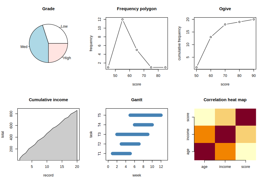
Step 2: The correlation matrix, as numbers
            age   income    score
age    1.000000 0.779453 0.508232
income 0.779453 1.000000 0.653628
score  0.508232 0.653628 1.000000
            age   income    score
age    1.000000 0.749531 0.408770
income 0.749531 1.000000 0.532175
score 0.408770 0.532175 1.000000The six diagrams are drawn above. Income is correlated 0.78 with age and 0.65 with score; age and score 0.51. The Spearman correlations are a little lower (0.75, 0.53, 0.41). Two rules matter more than any chart library: a pie chart with more than four or five slices cannot be read — use a bar chart; and a correlation matrix printed without its sample size says nothing — \(r = 0.5\) on twenty records and on two thousand are different findings.
Practical 5: Mathematical Model Building
1. Question
Model score on income; measure the fit three ways; compare polynomial models of increasing
degree by in-sample, 5-fold and leave-one-out cross-validated error; evaluate a hold-out split; and cross-tabulate
gender against grade.
2. Aim
To fit a model and then measure the gap between its fit to the data in hand and its fit to data it has not seen.
3. Steps
- Fit the straight line and measure it three ways.
Three error measures, three different divisors, three different numbers.
- Over-fitting and under-fitting, measured.
The folds are fixed by
seq_len(n) %% k, so every degree is scored on exactly the same partition. - A hold-out split, done properly.
The split comes before anything is estimated.
- Cross-tabs: gender against grade.
| Command or formula | What it does |
|---|---|
lm(y ~ x) | the least-squares fit; poly(x, d, raw = TRUE) for a polynomial of degree d |
| RMSE, MAE, \(\sigma\) | \(\sqrt{SSE/n}\); \(\frac1n\sum|e|\); \(\sqrt{SSE/(n-2)}\), the residual standard deviation |
| \(k\)-fold cross-validation | fit on \(k-1\) folds, predict the held-out fold, pool the errors; \(k = n\) is leave-one-out |
chisq.test(table), fisher.test(table) | the test of a cross-tab; Fisher's is exact, for small expected counts |
4. Programme
# Practical 5: Mathematical Model Building

# The data set: twenty records
customers <- data.frame(
  id     = 1:20,
  age    = c(23,45,31,58,27,39,52,34,29,48,36,41,25,55,33,44,30,50,28,38),
  income = c(40,57,37,69,36,38,63,32,35,57,42,49,26,39,48,49,23,57,27,33),
  score  = c(54,55,64,77,69,60,85,57,65,59,64,60,51,57,60,60,55,67,40,56),
  gender = factor(c("M","F","M","F","M","F","M","F","M","F",
                    "M","F","M","F","M","F","M","F","M","F")),
  buy    = c(0,1,0,1,1,0,1,0,0,1,0,0,0,0,1,1,0,1,0,0)
)
customers$grade <- cut(customers$score, breaks = c(-Inf, 57, 65, Inf),
                       labels = c("Low","Med","High"), right = FALSE)
customers$buy <- factor(customers$buy, levels = c(0,1), labels = c("No","Yes"))

# Step 1: Fit the straight line and measure it three ways
fit <- lm(score ~ income, data = customers)
coef(fit)
round(c(R2 = summary(fit)$r.squared, adjR2 = summary(fit)$adj.r.squared,
        RMSE = sqrt(mean(resid(fit)^2)), MAE = mean(abs(resid(fit))), sigma = summary(fit)$sigma), 6)

# Step 2: Over-fitting and under-fitting, measured
rmse <- function(y, yhat) sqrt(mean((y - yhat)^2))
cv <- function(d, k, degree = 1) {          # k-fold cross-validation, written out
  fold <- seq_len(nrow(d)) %% k
  sq <- c()
  for (f in unique(fold)) {
    tr <- d[fold != f, ]; te <- d[fold == f, ]
    mdl <- lm(score ~ poly(income, degree, raw = TRUE), data = tr)
    sq <- c(sq, (te$score - predict(mdl, te))^2)
  }
  sqrt(mean(sq))
}
deg <- c(1, 2, 3, 5, 8)
in_sample <- sapply(deg, function(g)
  rmse(customers$score, fitted(lm(score ~ poly(income, g, raw = TRUE), data = customers))))
data.frame(degree = deg, in_sample = round(in_sample, 4),
           cv5   = round(sapply(deg, function(g) cv(customers, 5, g)), 4),
           loocv = round(sapply(deg, function(g) cv(customers, nrow(customers), g)), 4))

# Step 3: A hold-out split, done properly
train <- customers[1:14, ]; test <- customers[15:20, ]
m <- lm(score ~ income, data = train)
coef(m)
round(c(train = rmse(train$score, predict(m, train)), test = rmse(test$score, predict(m, test))), 6)

# Step 4: Cross-tabs: gender against grade
tab <- table(customers$gender, customers$grade); tab
chisq.test(tab)
chisq.test(tab)$expected
round(prop.table(tab, 1), 3)
fisher.test(tab)$p.value
5. Execution and Results
Step 1: Fit the straight line and measure it three ways
(Intercept)      income
 40.1476548   0.4808015
      R2    adjR2     RMSE      MAE    sigma
0.427229 0.395409 6.960550 5.437054 7.337064
Step 2: Over-fitting and under-fitting, measured
  degree in_sample       cv5     loocv
1      1    6.9605    7.3777    7.9238
2      2    6.9053    7.5765    8.1354
3      3    6.3354   10.8021   10.7390
4      5    4.7282   17.7650   13.0146
5      8    3.7028 1305.5409 1793.8866
Step 3: A hold-out split, done properly
(Intercept)      income
 43.6770976   0.4282591
   train     test
7.229596 6.813509
Step 4: Cross-tabs: gender against grade
    Low Med High
  F   2   6    2
  M   4   3    3

	Pearson's Chi-squared test

data:  tab
X-squared = 1.8667, df = 2, p-value = 0.3932

Warning message:
In chisq.test(tab) :
  Chi-squared approximation may be incorrect

    Low Med High
  F   3 4.5  2.5
  M   3 4.5  2.5
Warning message:
In chisq.test(tab) :
  Chi-squared approximation may be incorrect

    Low Med High
  F 0.2 0.6  0.2
  M 0.4 0.3  0.3
[1] 0.5226136The straight line is \(\widehat{score} = 40.15 + 0.481\,income\), \(R^{2} = 0.427\). The in-sample error falls with every added degree — it must — while the cross-validated error rises from degree 2 and then explodes: by degree 8 the curve passes almost through the points and predicts a held-out point with an error in the hundreds, or thousands, on a scale whose whole range is 40 to 85. That divergence is over-fitting, and a model chosen by in-sample error alone would have chosen degree 8. The straight line is the model. On the hold-out split its error is 7.23 on the data fitted and 6.81 on data never seen. The gender × grade table gives \(\chi^{2} = 1.87\) on 2 d.f. (\(p = 0.39\)), but every expected count is below 5 and R warns: the approximation does not hold, and Fisher's exact test, \(p = 0.52\), is the one to quote — no evidence that grade depends on gender.
Practical 6: Evaluation of Model Performance
1. Question
Predict buy from income by logistic regression, classify at a fitted probability of 0.5, and
evaluate the classifier by its confusion matrix, the ratios from it, the no-information rate and the AUC.
2. Aim
To evaluate a classifier quantitatively and qualitatively, and to judge its accuracy against the rate a model-free guess would score.
3. Steps
- Fit the logistic regression.
- The confusion matrix.
- The ratios, and the no-information rate.
- The AUC, by the rank identity.
| Command or formula | What it does |
|---|---|
glm(y ~ x, family = binomial) | logistic regression; \(e^{b}\) is the odds ratio per unit of \(x\) |
| Accuracy, precision, recall | \((TP+TN)/n\); \(TP/(TP+FP)\); \(TP/(TP+FN)\) |
| Specificity, \(F_1\) | \(TN/(TN+FP)\); \(2PR/(P+R)\) |
| AUC | \(P(\hat p_{\text{Yes}} > \hat p_{\text{No}})\): the share of (Yes, No) pairs ranked the right way round |
| RMSE, MAE, \(R^{2}\), adjusted \(R^{2}\) | for a numeric prediction: RMSE squares, so one large error dominates; adjusted \(R^{2}\) can fall, and is the one to compare models with |
4. Programme
# Practical 6: Evaluation of Model Performance

# The data set: twenty records
customers <- data.frame(
  id     = 1:20,
  age    = c(23,45,31,58,27,39,52,34,29,48,36,41,25,55,33,44,30,50,28,38),
  income = c(40,57,37,69,36,38,63,32,35,57,42,49,26,39,48,49,23,57,27,33),
  score  = c(54,55,64,77,69,60,85,57,65,59,64,60,51,57,60,60,55,67,40,56),
  gender = factor(c("M","F","M","F","M","F","M","F","M","F",
                    "M","F","M","F","M","F","M","F","M","F")),
  buy    = c(0,1,0,1,1,0,1,0,0,1,0,0,0,0,1,1,0,1,0,0)
)
customers$grade <- cut(customers$score, breaks = c(-Inf, 57, 65, Inf),
                       labels = c("Low","Med","High"), right = FALSE)
customers$buy <- factor(customers$buy, levels = c(0,1), labels = c("No","Yes"))

# Step 1: Fit the logistic regression
g <- glm(buy ~ income, data = customers, family = binomial)
coef(g)
exp(coef(g)["income"])            # the odds multiply by this per unit of income
-coef(g)[1] / coef(g)[2]           # the income at which the fitted probability is 1/2

# Step 2: The confusion matrix
p    <- predict(g, type = "response")
pred <- factor(ifelse(p >= 0.5, "Yes", "No"), levels = c("No", "Yes"))
cm <- table(Predicted = pred, Actual = customers$buy); cm

# Step 3: The ratios, and the no-information rate
TP <- cm["Yes","Yes"]; TN <- cm["No","No"]; FP <- cm["Yes","No"]; FN <- cm["No","Yes"]
prec <- TP/(TP + FP); rec <- TP/(TP + FN)
round(c(accuracy = (TP + TN)/sum(cm), precision = prec, recall = rec,
        specificity = TN/(TN + FP), F1 = 2*prec*rec/(prec + rec),
        no_information = max(table(customers$buy))/nrow(customers)), 6)

# Step 4: The AUC, by the rank identity
pos <- p[customers$buy == "Yes"]; neg <- p[customers$buy == "No"]
mean(outer(pos, neg, function(a, b) (a > b) + 0.5*(a == b)))   # over 8 x 12 = 96 pairs
5. Execution and Results
Step 1: Fit the logistic regression
(Intercept)      income
-11.4011323   0.2501235
  income
1.284184
(Intercept)
   45.58201
Step 2: The confusion matrix
         Actual
Predicted No Yes
      No  11   1
      Yes  1   7
Step 3: The ratios, and the no-information rate
      accuracy      precision         recall    specificity
      0.900000       0.875000       0.875000       0.916667
            F1 no_information
      0.875000       0.600000
Step 4: The AUC, by the rank identity
[1] 0.921875The odds of buying multiply by 1.28 per unit of income, and the fitted probability passes 1/2 at an income of 45.6. At that threshold the classifier gets 18 of 20 right: accuracy 0.90, precision and recall 0.875, specificity 0.917, \(F_1\) 0.875, AUC 0.922. Accuracy on its own is the trap: predicting No for everyone scores 0.60, the no-information rate, so 0.90 against 0.60 is a real gain — and the same 0.90 against a base rate of 0.95 would be a failure. Precision and recall move in opposite directions as the threshold moves; AUC does not depend on it, which is why it is the one to compare models with.
Practical 7: Parametric Tests
1. Question
Compare score between men and women by the variance-ratio test and the two-sample \(t\) test, in that
order, and analyse score by grade by one-way analysis of variance.
2. Aim
To run the parametric tests in the order they depend on each other, and to recognise a test that cannot fail.
3. Steps
- The two groups.
- 1. The variances first, because the next test depends on the answer.
- 2. The means.
- 3. More than two groups: one-way analysis of variance.
| Command or formula | What it does |
|---|---|
var.test(x, y) | \(F = s_1^{2}/s_2^{2}\) on \((n_1-1, n_2-1)\) d.f. |
t.test(x, y, var.equal = TRUE) | the pooled two-sample \(t\), justified only if the variances may be pooled |
aov(y ~ g) | one-way analysis of variance |
4. Programme
# Practical 7: Parametric Tests

# The data set: twenty records
customers <- data.frame(
  id     = 1:20,
  age    = c(23,45,31,58,27,39,52,34,29,48,36,41,25,55,33,44,30,50,28,38),
  income = c(40,57,37,69,36,38,63,32,35,57,42,49,26,39,48,49,23,57,27,33),
  score  = c(54,55,64,77,69,60,85,57,65,59,64,60,51,57,60,60,55,67,40,56),
  gender = factor(c("M","F","M","F","M","F","M","F","M","F",
                    "M","F","M","F","M","F","M","F","M","F")),
  buy    = c(0,1,0,1,1,0,1,0,0,1,0,0,0,0,1,1,0,1,0,0)
)
customers$grade <- cut(customers$score, breaks = c(-Inf, 57, 65, Inf),
                       labels = c("Low","Med","High"), right = FALSE)
customers$buy <- factor(customers$buy, levels = c(0,1), labels = c("No","Yes"))

# Step 1: The two groups
M <- customers$score[customers$gender == "M"]
F <- customers$score[customers$gender == "F"]
M; F
round(c(mean_M = mean(M), mean_F = mean(F), var_M = var(M), var_F = var(F)), 2)

# Step 2: 1. The variances first, because the next test depends on the answer
var.test(M, F)

# Step 3: 2. The means
t.test(M, F, var.equal = TRUE)

# Step 4: 3. More than two groups: one-way analysis of variance
summary(aov(score ~ grade, data = customers))
5. Execution and Results
Step 1: The two groups
 [1] 54 64 69 85 65 64 51 60 55 40
 [1] 55 77 60 57 59 60 57 60 67 56
mean_M mean_F  var_M  var_F
 60.70  60.80 144.46  43.51
Step 2: 1. The variances first, because the next test depends on the answer
	F test to compare two variances

data:  M and F
F = 3.32, num df = 9, denom df = 9, p-value = 0.08848
alternative hypothesis: true ratio of variances is not equal to 1
95 percent confidence interval:
  0.8246334 13.3661772
sample estimates:
ratio of variances
          3.319969
Step 3: 2. The means
	Two Sample t-test

data:  M and F
t = -0.023065, df = 18, p-value = 0.9819
alternative hypothesis: true difference in means is not equal to 0
95 percent confidence interval:
 -9.208573  9.008573
sample estimates:
mean of x mean of y
     60.7      60.8
Step 4: 3. More than two groups: one-way analysis of variance
            Df Sum Sq Mean Sq F value   Pr(>F)
grade        2 1182.8   591.4   19.76 3.68e-05 ***
Residuals   17  508.9    29.9
---
Signif. codes: 0 ‘***’ 0.001 ‘**’ 0.01 ‘*’ 0.05 ‘.’ 0.1 ‘ ’ 1The variance ratio is 3.32 on (9, 9) d.f., \(p = 0.088\): not significant, so pooling is defensible. The pooled
\(t\) is −0.023 on 18 d.f., \(p = 0.98\): the group means, 60.7 and 60.8, are as close to equal as twenty numbers are
likely to come. What differs is the spread — variances 144.46 and 43.51 — which a test of means would have
missed, and which is why the variance test comes first and is reported whatever it says. The analysis of
variance by grade proves nothing: \(F = 19.76\), \(p = 0.000037\), looks decisive and is circular, because
grade was derived from score; testing a variable against a grouping built out of it always
succeeds.
Practical 8: Non-Parametric Tests
1. Question
Twelve subjects are measured before and after a training programme:
| before | 68, 72, 65, 70, 74, 66, 71, 69, 73, 67, 75, 64 |
|---|---|
| after | 71, 74, 64, 73, 77, 69, 70, 72, 76, 71, 74, 68 |
Test for a change by the sign test and the Wilcoxon signed-rank test. On customers, compare
score between men and women by the Mann–Whitney and median tests, and test the residuals of
score ~ income for independence by the runs test.
2. Aim
To apply five non-parametric tests and see how much each uses of the data.
3. Steps
- The differences.
- Sign test: 9 positive, 3 negative, no ties.
- Wilcoxon signed rank, using the magnitudes.
- Mann–Whitney U on score by gender.
- Mood's median test, on the same two groups.
- Runs test on the signs of the regression residuals.
| Command or formula | What it does |
|---|---|
| Sign test | paired; only the signs of the differences: binom.test(k, n, 0.5) |
| Wilcoxon signed rank | paired; signs and ranks of the magnitudes: wilcox.test(x, y, paired = TRUE) |
| Mann–Whitney \(U\) | two independent groups; ranks of the pooled sample: wilcox.test(x, y) |
| Median test | two or more groups; only above or below the grand median: \(\chi^{2}\) on the 2 × 2 table |
| Runs test | one ordered sequence; the number of runs of like signs; tests independence |
4. Programme
# Practical 8: Non-Parametric Tests

# The data set: twenty records
customers <- data.frame(
  id     = 1:20,
  age    = c(23,45,31,58,27,39,52,34,29,48,36,41,25,55,33,44,30,50,28,38),
  income = c(40,57,37,69,36,38,63,32,35,57,42,49,26,39,48,49,23,57,27,33),
  score  = c(54,55,64,77,69,60,85,57,65,59,64,60,51,57,60,60,55,67,40,56),
  gender = factor(c("M","F","M","F","M","F","M","F","M","F",
                    "M","F","M","F","M","F","M","F","M","F")),
  buy    = c(0,1,0,1,1,0,1,0,0,1,0,0,0,0,1,1,0,1,0,0)
)
customers$grade <- cut(customers$score, breaks = c(-Inf, 57, 65, Inf),
                       labels = c("Low","Med","High"), right = FALSE)
customers$buy <- factor(customers$buy, levels = c(0,1), labels = c("No","Yes"))

# Step 1: The differences
before <- c(68,72,65,70,74,66,71,69,73,67,75,64)
after  <- c(71,74,64,73,77,69,70,72,76,71,74,68)
d <- after - before; d

# Step 2: Sign test: 9 positive, 3 negative, no ties
binom.test(sum(d > 0), sum(d != 0), 0.5)$p.value

# Step 3: Wilcoxon signed rank, using the magnitudes
wilcox.test(after, before, paired = TRUE, correct = FALSE)

# Step 4: Mann–Whitney U on score by gender
M <- customers$score[customers$gender == "M"]
F <- customers$score[customers$gender == "F"]
wilcox.test(M, F, correct = FALSE)

# Step 5: Mood's median test, on the same two groups
gm <- median(customers$score); gm
tab <- table(customers$gender, customers$score > gm); tab
chisq.test(tab, correct = FALSE)

# Step 6: Runs test on the signs of the regression residuals
r <- resid(lm(score ~ income, data = customers))
s <- r > 0
runs <- 1 + sum(s[-1] != s[-length(s)])
n1 <- sum(s); n0 <- sum(!s)
mu <- 2*n1*n0/(n1 + n0) + 1
sg <- sqrt(2*n1*n0*(2*n1*n0 - n1 - n0) / ((n1 + n0)^2 * (n1 + n0 - 1)))
z <- (runs - mu)/sg
round(c(runs = runs, positive = n1, negative = n0, expected = mu, sd = sg, z = z, p = 2*pnorm(-abs(z))), 6)
5. Execution and Results
Step 1: The differences
[1] 3 2 -1 3 3 3 -1 3 3 4 -1 4Step 2: Sign test: 9 positive, 3 negative, no ties
[1] 0.1459961Step 3: Wilcoxon signed rank, using the magnitudes
	Wilcoxon signed rank test

data:  after and before
V = 72, p-value = 0.008551
alternative hypothesis: true location shift is not equal to 0

Warning message:
In wilcox.test.default(after, before, paired = TRUE, correct = FALSE) :
  cannot compute exact p-value with ties
Step 4: Mann–Whitney U on score by gender
	Wilcoxon rank sum test

data:  M and F
W = 50, p-value = 1
alternative hypothesis: true location shift is not equal to 0

Warning message:
In wilcox.test.default(M, F, correct = FALSE) :
  cannot compute exact p-value with ties
Step 5: Mood's median test, on the same two groups
[1] 60

    FALSE TRUE
  F     8    2
  M     5    5

	Pearson's Chi-squared test

data:  tab
X-squared = 1.978, df = 1, p-value = 0.1596

Warning message:
In chisq.test(tab, correct = FALSE) :
  Chi-squared approximation may be incorrect
Step 6: Runs test on the signs of the regression residuals
     runs  positive  negative  expected        sd         z         p
7.000000 9.000000 11.000000 10.900000 2.153455 -1.811043 0.070134 correct = FALSE R uses the normal approximation without a continuity correction; the default applies one and gives a slightly larger \(p\). Ties make R warn that an exact \(p\) cannot be computed, and R also corrects the variance of the statistic for the ties: for the training data \(W^{+} = 72\), \(W^{-} = 6\) (\(72 + 6 = 78 = n(n+1)/2\)), and the untied textbook standard deviation 12.75 would give \(p = 0.0096\), where R's tie-corrected one gives 0.0086.
Same data, same hypothesis: the sign test gives \(p = 0.146\) and the Wilcoxon \(p = 0.0086\). The three negative differences are all −1, the smallest magnitude present, while the nine positives run from 2 to 4; the sign test throws that away and counts 9 against 3, the Wilcoxon keeps it. Using only the signs costs real power. For score by gender, Mann–Whitney gives \(U\) exactly at its null mean (\(p = 1\)), agreeing with the \(t\) test of Practical 7; the median test, which keeps only one bit per value, gives \(p = 0.16\). The residuals form 7 runs where 10.9 were expected (\(p = 0.070\)): not significant at 5%, but close enough that the straight line should not be accepted without a plot of residuals against fitted values. The runs test is the one test here with no parametric counterpart — it tests independence, which every other test assumes.
Writing the Statistical Report
- Objective. One sentence: what question the data is being asked.
- The data. Source, number of records, every variable named with its scale, and the period or population it covers.
- Pre-processing. Missing values found and what was done about them; outliers found and whether they were kept; every transformation applied, with its reason. A reader who cannot reproduce your data frame cannot check anything else.
- Descriptive summary. A table of the summaries permitted by each variable's scale, and the two or three diagrams that carry the message.
- Analysis. Each test with its hypothesis, statistic, degrees of freedom, \(p\) value and conclusion in words — in that order, and its assumptions checked before it, not after.
- Model, if one was fitted. The equation, the coefficients with standard errors, the fit measures, and the out-of-sample error. An in-sample \(R^{2}\) reported alone is not a model evaluation.
- Conclusion and limitations. What the data supports, and what it does not. Twenty records support very little, and saying so is part of the answer.
- The code. Complete enough to run, with the seed if anything was random.
How Marks Are Lost
- Taking the mean of an ordinal variable. R will do it if the factor is not declared ordered. Declare it, and let R refuse.
- Scaling before splitting. The test set's mean and standard deviation then enter the training set, and the reported error is optimistic by an amount nobody can measure.
- Reporting an in-sample \(R^{2}\) as if it were a prediction error. Degree 8 in Practical 5 has the best in-sample fit and by far the worst prediction.
- Quoting accuracy without the no-information rate. \(0.90\) is good here and would be bad on a data set that is \(95\%\) one class.
- Ignoring R's expected-count warning on a \(\chi^{2}\) test. Pool the classes or use Fisher's exact test.
- Running a pooled \(t\) test without testing the variances first, or running it and not reporting the variance test because it came out inconvenient.
- Testing a variable against a grouping derived from it. The \(F = 19.76\) of Practical 7 is a worked example of an answer that cannot fail and means nothing.
- Not naming the convention. Type 7 quantiles, \(n-1\) in
sd, the continuity correction inwilcox.test: each changes the number, and a number whose convention is unstated cannot be reproduced.
What the Practical Record Should Contain
- 1. Question — the variables involved, with their measurement scales, and the pre-processing already applied.
- 2. Aim — in one line.
- 3. Steps — the method, the assumptions it requires and the check made on each, with the R commands used.
- 4. Programme — the R, complete enough to run.
- 5. Execution and Results — the output, with the statistic, its degrees of freedom and the \(p\) value; a second route to the same answer where one exists (the parametric test beside its non-parametric counterpart, or the identity \(W^{+} + W^{-} = n(n+1)/2\)); and the conclusion in words, with what it does not establish.