R Programming — Practical Course

How to use this manual: in the lab, copy the programme into an R script and run it line by line; the output you should see is under Execution and Results, step by step, with the result at the end. Every output and plot on this page was produced by running the programme shown, in R 4.3.3. Use the built-in datasets (iris, mtcars, airquality, sleep) or a CSV from the UCI ML Repository.

List of Practical Experiments (Official Syllabus)

Data Import and Preprocessing — import dataset (e.g., iris), handle missing values, basic sub-setting.
Descriptive Statistics Computation — mean, variance, skewness; interpret results.
Frequency Analysis — contingency tables and chi-square tests on categorical data.
Basic Visualizations — histograms and boxplots to assess data normality.
Hypothesis Testing — t-tests and ANOVA on experimental data, reporting p-values.
Non-Parametric Tests — Wilcoxon tests; compare with parametric alternatives.
Linear Regression Modeling — fit a simple linear model, plot residuals, predict new values.

Experiment 1: Data Import & Preprocessing

1. Question

Import the built-in airquality dataset (153 observations, 6 variables), examine its structure, count and handle the missing values, and create subsets.

2. Aim

To read a dataset into R, inspect it, deal with missing values (drop or impute), and perform sub-setting.

3. Steps

Load the data and inspect its structure.
Count the missing values in each column.
Drop the rows with any missing value.
Or mean-impute Ozone, keeping every row.
A copy, aq, is imputed, so that airquality itself is left as it was loaded.
Subset the hot days.
Save the cleaned file.

R COMMANDS AND FORMULAS USED

Command or formula	What it does
`data()`, `str()`	load a built-in dataset; show its structure
`colSums(is.na(d))`	the number of missing values in each column
`na.omit(d)`	drops every row with a missing value
`d$v[is.na(d$v)] <- mean(d$v, na.rm = TRUE)`	replaces the missing values by the mean (mean-imputation)
`subset(d, condition)`	the rows meeting a condition
`write.csv(d, file, row.names = FALSE)`	saves a data frame as a CSV file

4. Programme

EXPERIMENT 1 — THE R PROGRAMME

# Experiment 1: Data Import & Preprocessing

# Step 1: Load the data and inspect its structure
data(airquality)
str(airquality)

# Step 2: Count the missing values in each column
colSums(is.na(airquality))

# Step 3: Drop the rows with any missing value
clean <- na.omit(airquality)
nrow(clean)

# Step 4: Or mean-impute Ozone, keeping every row
aq <- airquality
aq$Ozone[is.na(aq$Ozone)] <- mean(aq$Ozone, na.rm = TRUE)
colSums(is.na(aq))

# Step 5: Subset the hot days
hot <- subset(aq, Temp > 80)
nrow(hot)

# Step 6: Save the cleaned file
write.csv(clean, "airquality_clean.csv", row.names = FALSE)

5. Execution and Results

Step 1: Load the data and inspect its structure

OUTPUT

'data.frame':	153 obs. of  6 variables:
 $ Ozone  : int  41 36 12 18 NA 28 23 19 8 NA ...
 $ Solar.R: int  190 118 149 313 NA NA 299 99 19 194 ...
 $ Wind   : num  7.4 8 12.6 11.5 14.3 14.9 8.6 13.8 20.1 8.6 ...
 $ Temp   : int  67 72 74 62 56 66 65 59 61 69 ...
 $ Month  : int  5 5 5 5 5 5 5 5 5 5 ...
 $ Day    : int  1 2 3 4 5 6 7 8 9 10 ...

Step 2: Count the missing values in each column

OUTPUT

  Ozone Solar.R    Wind    Temp   Month     Day 
     37       7       0       0       0       0

Step 3: Drop the rows with any missing value

OUTPUT

[1] 111

Step 4: Or mean-impute Ozone, keeping every row

OUTPUT

  Ozone Solar.R    Wind    Temp   Month     Day 
      0       7       0       0       0       0

Step 5: Subset the hot days

OUTPUT

[1] 68

Step 6: Save the cleaned file

Nothing is printed: write.csv() writes the file airquality_clean.csv into the working directory.

RESULT

The dataset has 153 rows, with 37 missing values in Ozone and 7 in Solar.R; na.omit leaves 111 complete rows, while mean-imputing Ozone keeps all 153 (Solar.R still has its 7). There are 68 days hotter than 80°F. The cleaned data are saved for later experiments.

Experiment 2: Descriptive Statistics

1. Question

For iris$Sepal.Length (150 observations), compute the standard descriptive statistics and the shape measures (skewness, kurtosis), then interpret.

2. Aim

To summarise a numeric variable in R with measures of location, dispersion and shape.

3. Steps

Location and dispersion.
Skewness and kurtosis, from the moments.
The central moments are computed directly; moments::skewness() and moments::kurtosis() use the same formulas.
A fuller report (optional).
summary(x) is in base R; the psych package's describe(x) adds more.

R COMMANDS AND FORMULAS USED

Command or formula	What it does
`mean median var sd range IQR`	location and dispersion; `var` and `sd` divide by $n-1$
Skewness	$\sqrt{b_1} = m_3/m_2^{3/2}$, with $m_k = \frac1n\sum(x - \bar x)^{k}$
Kurtosis	$b_2 = m_4/m_2^{2}$; 3 for a normal curve

4. Programme

EXPERIMENT 2 — THE R PROGRAMME

# Experiment 2: Descriptive Statistics

# Step 1: Location and dispersion
data(iris); x <- iris$Sepal.Length
c(mean = mean(x), median = median(x), var = var(x), sd = sd(x), IQR = IQR(x))
range(x)

# Step 2: Skewness and kurtosis, from the moments
m <- function(k) mean((x - mean(x))^k)     # k-th central moment
c(skewness = m(3) / m(2)^1.5, kurtosis = m(4) / m(2)^2)

# Step 3: A fuller report (optional)
summary(x)

5. Execution and Results

Step 1: Location and dispersion

OUTPUT

     mean    median       var        sd       IQR 
5.8433333 5.8000000 0.6856935 0.8280661 1.3000000 
[1] 4.3 7.9

Step 2: Skewness and kurtosis, from the moments

OUTPUT

 skewness  kurtosis 
0.3117531 2.4264321

Step 3: A fuller report (optional)

OUTPUT

   Min. 1st Qu.  Median    Mean 3rd Qu.    Max. 
  4.300   5.100   5.800   5.843   6.400   7.900

Note. The moments package gives skewness() and kurtosis(); where it is not installed, the two lines above compute the same values from the central moments.

RESULT

Sepal.Length has mean 5.84 cm, median 5.80 and standard deviation 0.83 (variance 0.686, IQR 1.3). It is mildly right-skewed (skewness 0.31 > 0) and platykurtic (kurtosis 2.43 < 3): slightly flatter than a normal curve.

Experiment 3: Frequency Analysis & Chi-Square

1. Question

Cross-classify iris flowers by Species and by whether the petal is "Long" (Petal.Length > 4) or "Short", and test whether Species and petal category are independent. As a variant, test 120 simulated rolls of a die for fairness.

2. Aim

To build a contingency table and apply the chi-square test of independence, and a goodness-of-fit test.

3. Steps

Make the petal category and the two-way table.
Test independence.
Goodness of fit: 120 simulated rolls of a die.

R COMMANDS AND FORMULAS USED

Command or formula	What it does
`ifelse(cond, a, b)`	makes a categorical variable from a condition
`table(f1, f2)`	the contingency table of counts
`chisq.test(tbl)`	$\chi^2 = \sum (O-E)^2/E$ on $(r-1)(c-1)$ d.f.; on a one-way table, against equal probabilities

4. Programme

EXPERIMENT 3 — THE R PROGRAMME

# Experiment 3: Frequency Analysis & Chi-Square

# Step 1: Make the petal category and the two-way table
big <- ifelse(iris$Petal.Length > 4, "Long", "Short")
tbl <- table(iris$Species, big); tbl

# Step 2: Test independence
chisq.test(tbl)

# Step 3: Goodness of fit: 120 simulated rolls of a die
set.seed(7); rolls <- sample(1:6, 120, replace = TRUE)
table(rolls)
chisq.test(table(rolls))        # expected: 20 of each

5. Execution and Results

Step 1: Make the petal category and the two-way table

OUTPUT

            big
             Long Short
  setosa        0    50
  versicolor   34    16
  virginica    50     0

Step 2: Test independence

OUTPUT


	Pearson's Chi-squared test

data:  tbl
X-squared = 105.84, df = 2, p-value < 2.2e-16

Step 3: Goodness of fit: 120 simulated rolls of a die

OUTPUT

rolls
 1  2  3  4  5  6 
18 25 19 20 18 20 

	Chi-squared test for given probabilities

data:  table(rolls)
X-squared = 1.7, df = 5, p-value = 0.8889

RESULT

$\chi^2 = 105.84$ on 2 d.f., $p < 2.2 \times 10^{-16}$: independence is rejected — petal category is strongly associated with species (every setosa is "Short", every virginica "Long"). For the die, $\chi^2 = 1.7$ on 5 d.f., $p = 0.89$: the simulated rolls are consistent with a fair die.

Experiment 4: Basic Visualizations & Normality

1. Question

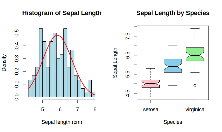
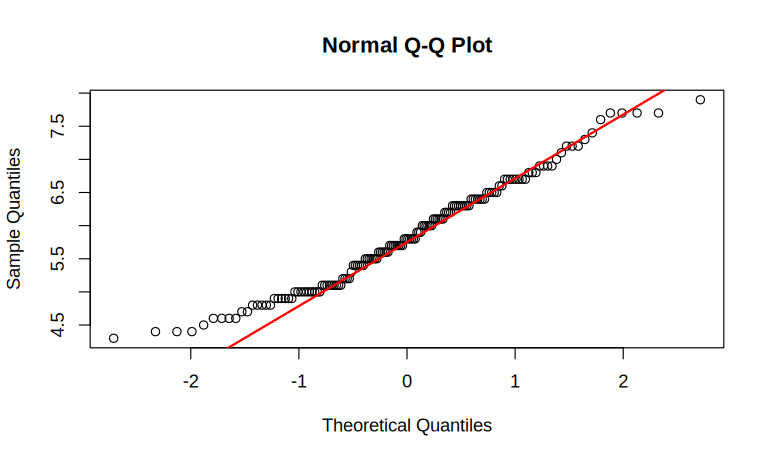
Visualise iris variables with histograms and boxplots, and assess the normality of Sepal.Length with a Q-Q plot and the Shapiro–Wilk test.

2. Aim

To produce diagnostic plots and a formal normality test to judge whether a variable is normally distributed.

3. Steps

Histogram with the normal curve, and boxplots by species.
The Q-Q plot.
The Shapiro–Wilk test.

R COMMANDS AND FORMULAS USED

Command or formula	What it does
`hist(x, freq = FALSE)`, `curve(dnorm(x, m, s), add = TRUE)`	a density histogram with the fitted normal curve over it
`boxplot(y ~ group)`	one box per group
`qqnorm(x)`, `qqline(x)`	the normal Q-Q plot and its reference line
`shapiro.test(x)`	the Shapiro–Wilk test of $H_0$: normal

4. Programme

EXPERIMENT 4 — THE R PROGRAMME

# Experiment 4: Basic Visualizations & Normality

# Step 1: Histogram with the normal curve, and boxplots by species
par(mfrow = c(1, 2))
hist(iris$Sepal.Length, breaks = 15, col = "lightblue", freq = FALSE,
     main = "Histogram of Sepal Length", xlab = "Sepal length (cm)")
curve(dnorm(x, mean(iris$Sepal.Length), sd(iris$Sepal.Length)), add = TRUE, col = "red", lwd = 2)
boxplot(Sepal.Length ~ Species, data = iris, notch = TRUE,
        col = c("pink", "skyblue", "lightgreen"), main = "Sepal Length by Species")
par(mfrow = c(1, 1))

# Step 2: The Q-Q plot
qqnorm(iris$Sepal.Length); qqline(iris$Sepal.Length, col = "red", lwd = 2)

# Step 3: The Shapiro–Wilk test
shapiro.test(iris$Sepal.Length)

5. Execution and Results

Step 1: Histogram with the normal curve, and boxplots by species

PLOT

Experiment 4: Histogram with the normal curve, and boxplots by species, as drawn by the R code above

Step 2: The Q-Q plot

PLOT

Experiment 4: The Q-Q plot, as drawn by the R code above

Step 3: The Shapiro–Wilk test

OUTPUT


	Shapiro-Wilk normality test

data:  iris$Sepal.Length
W = 0.97609, p-value = 0.01018

RESULT

The histogram is roughly bell-shaped, the boxplots show Sepal.Length rising from setosa to virginica (with one low virginica value), and the Q-Q points follow the line except in the tails. Shapiro–Wilk gives $W = 0.976$, $p = 0.0102$, just below 0.05: normality is borderline — a caution to consider the non-parametric tests of Experiment 6.

Choosing the Right Test (Experiments 3, 5, 6, 7)

The decision every lab report should make explicit: what the question is, whether assumptions hold, and which R function follows. Quote this reasoning in the Interpretation section of your notebook.

Experiment 5: Hypothesis Testing (t-tests & ANOVA)

1. Question

Carry out (a) a one-sample t-test of $H_0:\mu = 50$ on ten measurements, (b) a two-sample (Welch) t-test comparing setosa and versicolor Sepal.Length, (c) a paired t-test on the sleep data, and (d) a one-way ANOVA of Sepal.Length by Species, with Tukey's comparisons.

2. Aim

To perform parametric tests of means (one-sample, two-sample, paired) and ANOVA in R and report the p-values.

3. Steps

(a) One-sample t-test.
(b) Two-sample Welch t-test.
(c) Paired t-test on sleep.
The two groups of sleep are the same ten patients, so the test is paired.
(d) One-way ANOVA and Tukey's comparisons.

R COMMANDS AND FORMULAS USED

Command or formula	What it does
`t.test(x, mu = m0)`	one-sample: $t = (\bar x - \mu_0)/(s/\sqrt n)$
`t.test(x, y)`	two-sample, Welch (unequal variances) by default
`t.test(x, y, paired = TRUE)`	paired: a one-sample test on the differences
`aov(y ~ group)`, `TukeyHSD()`	one-way ANOVA, $F = MS_{between}/MS_{within}$, and all pairwise comparisons

4. Programme

EXPERIMENT 5 — THE R PROGRAMME

# Experiment 5: Hypothesis Testing (t-tests & ANOVA)

# Step 1: (a) One-sample t-test
x <- c(48, 52, 49, 53, 51, 47, 55, 50, 49, 52)
t.test(x, mu = 50)

# Step 2: (b) Two-sample Welch t-test
setosa     <- iris$Sepal.Length[iris$Species == "setosa"]
versicolor <- iris$Sepal.Length[iris$Species == "versicolor"]
t.test(setosa, versicolor)

# Step 3: (c) Paired t-test on sleep
data(sleep)
with(sleep, t.test(extra[group == 1], extra[group == 2], paired = TRUE))

# Step 4: (d) One-way ANOVA and Tukey's comparisons
fit <- aov(Sepal.Length ~ Species, data = iris)
summary(fit)
TukeyHSD(fit)

5. Execution and Results

Step 1: (a) One-sample t-test

OUTPUT


	One Sample t-test

data:  x
t = 0.77174, df = 9, p-value = 0.46
alternative hypothesis: true mean is not equal to 50
95 percent confidence interval:
 48.84126 52.35874
sample estimates:
mean of x 
     50.6

Step 2: (b) Two-sample Welch t-test

OUTPUT


	Welch Two Sample t-test

data:  setosa and versicolor
t = -10.521, df = 86.538, p-value < 2.2e-16
alternative hypothesis: true difference in means is not equal to 0
95 percent confidence interval:
 -1.1057074 -0.7542926
sample estimates:
mean of x mean of y 
    5.006     5.936

Step 3: (c) Paired t-test on sleep

OUTPUT


	Paired t-test

data:  extra[group == 1] and extra[group == 2]
t = -4.0621, df = 9, p-value = 0.002833
alternative hypothesis: true mean difference is not equal to 0
95 percent confidence interval:
 -2.4598858 -0.7001142
sample estimates:
mean difference 
          -1.58

Step 4: (d) One-way ANOVA and Tukey's comparisons

OUTPUT

             Df Sum Sq Mean Sq F value Pr(>F)    
Species       2  63.21  31.606   119.3 <2e-16 ***
Residuals   147  38.96   0.265                   
---
Signif. codes:  0 ‘***’ 0.001 ‘**’ 0.01 ‘*’ 0.05 ‘.’ 0.1 ‘ ’ 1
  Tukey multiple comparisons of means
    95% family-wise confidence level

Fit: aov(formula = Sepal.Length ~ Species, data = iris)

$Species
                      diff       lwr       upr p adj
versicolor-setosa    0.930 0.6862273 1.1737727     0
virginica-setosa     1.582 1.3382273 1.8257727     0
virginica-versicolor 0.652 0.4082273 0.8957727     0

Note. The paired test is written with two vectors. The formula form t.test(extra ~ group, data = sleep, paired = TRUE) works in older versions of R but is refused from R 4.4.0 onwards; the two-vector form works in every version.

RESULT

(a) The ten measurements are consistent with $\mu = 50$ ($t = 0.77$, $p = 0.46$). (b) Setosa and versicolor differ strongly ($t = -10.52$, $p < 2.2 \times 10^{-16}$). (c) The drug has a significant paired effect ($t = -4.06$, 9 d.f., $p = 0.0028$). (d) The species means differ ($F = 119.3$, $p < 2 \times 10^{-16}$), and Tukey's comparisons show all three pairs different.

Experiment 6: Non-Parametric Tests

1. Question

Repeat the location comparisons of Experiment 5 without the normality assumption: a one-sample Wilcoxon signed-rank test, a paired signed-rank test on sleep, and a Wilcoxon rank-sum (Mann–Whitney) test for setosa against versicolor; compare the last with its parametric counterpart.

2. Aim

To apply rank-based non-parametric tests and contrast them with the parametric t-tests.

3. Steps

One-sample signed-rank test.
Paired signed-rank test on sleep.
Rank-sum test, setosa against versicolor.
The two p-values side by side.

R COMMANDS AND FORMULAS USED

Command or formula	What it does
`wilcox.test(x, mu = m0)`	one-sample signed-rank test
`wilcox.test(x, y, paired = TRUE)`	paired signed-rank test
`wilcox.test(x, y)`	rank-sum (Mann–Whitney) test

4. Programme

EXPERIMENT 6 — THE R PROGRAMME

# Experiment 6: Non-Parametric Tests

# Step 1: One-sample signed-rank test
x <- c(48, 52, 49, 53, 51, 47, 55, 50, 49, 52)
wilcox.test(x, mu = 50)

# Step 2: Paired signed-rank test on sleep
with(sleep, wilcox.test(extra[group == 1], extra[group == 2], paired = TRUE))

# Step 3: Rank-sum test, setosa against versicolor
setosa     <- iris$Sepal.Length[iris$Species == "setosa"]
versicolor <- iris$Sepal.Length[iris$Species == "versicolor"]
wilcox.test(setosa, versicolor)

# Step 4: The two p-values side by side
data.frame(Test = c("Welch t", "Wilcoxon rank-sum"),
           p = c(t.test(setosa, versicolor)$p.value, suppressWarnings(wilcox.test(setosa, versicolor)$p.value)))

5. Execution and Results

Step 1: One-sample signed-rank test

OUTPUT


	Wilcoxon signed rank test with continuity correction

data:  x
V = 28.5, p-value = 0.5113
alternative hypothesis: true location is not equal to 50

Warning messages:
1: In wilcox.test.default(x, mu = 50) :
  cannot compute exact p-value with ties
2: In wilcox.test.default(x, mu = 50) :
  cannot compute exact p-value with zeroes

Step 2: Paired signed-rank test on sleep

OUTPUT


	Wilcoxon signed rank test with continuity correction

data:  extra[group == 1] and extra[group == 2]
V = 0, p-value = 0.009091
alternative hypothesis: true location shift is not equal to 0

Warning messages:
1: In wilcox.test.default(extra[group == 1], extra[group == 2], paired = TRUE) :
  cannot compute exact p-value with ties
2: In wilcox.test.default(extra[group == 1], extra[group == 2], paired = TRUE) :
  cannot compute exact p-value with zeroes

Step 3: Rank-sum test, setosa against versicolor

OUTPUT


	Wilcoxon rank sum test with continuity correction

data:  setosa and versicolor
W = 168.5, p-value = 8.346e-14
alternative hypothesis: true location shift is not equal to 0

Step 4: The two p-values side by side

OUTPUT

               Test            p
1           Welch t 3.746743e-17
2 Wilcoxon rank-sum 8.345827e-14

Note. The data contain ties (and, in the one-sample case, a value equal to 50), so R cannot compute exact p-values and says so in its warnings; it uses the normal approximation with a continuity correction instead.

RESULT

The non-parametric tests agree with the parametric ones: no shift from 50 in the one-sample case ($V = 28.5$, $p = 0.51$); a significant paired effect on sleep ($p = 0.009$); and a strong setosa–versicolor difference ($W = 168.5$, $p = 8.3 \times 10^{-14}$, against Welch's $3.7 \times 10^{-17}$). Wilcoxon is preferred when normality is doubtful, as Experiment 4 flagged.

Experiment 7: Linear Regression Modeling

1. Question

Using mtcars, model fuel economy (mpg) as a linear function of weight (wt), check the residuals, and predict mpg for weights 2.5, 3.5 and 4.5 (thousand lb).

2. Aim

To fit a simple linear regression, assess it (R², residual diagnostics) and forecast with prediction intervals.

3. Steps

Fit the model.
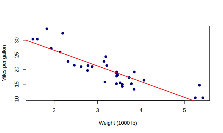
The scatter with the fitted line.
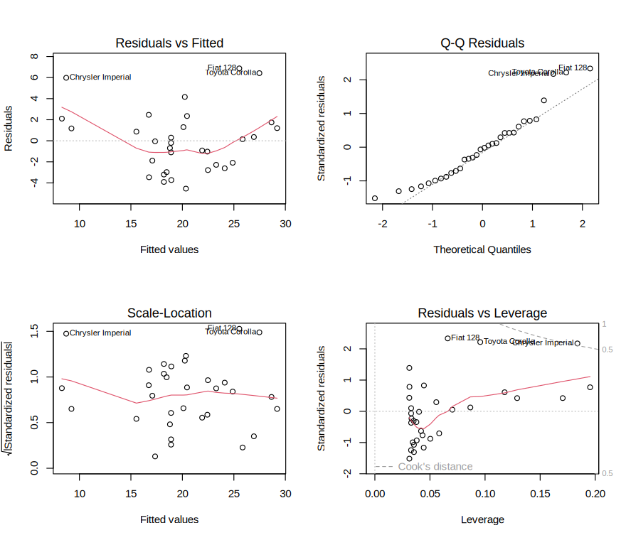
The residual diagnostics.
Normality of the residuals.
Predict at 2.5, 3.5 and 4.5.

R COMMANDS AND FORMULAS USED

Command or formula	What it does
`lm(y ~ x)`, `summary(fit)`	fit $\hat y = a + bx$, $b = S_{xy}/S_{xx}$; coefficients, $R^2$, tests
`plot(fit)`	the four residual diagnostic plots
`shapiro.test(resid(fit))`	normality of the residuals
`predict(fit, newdata, interval = "prediction")`	predictions with 95% prediction intervals

4. Programme

EXPERIMENT 7 — THE R PROGRAMME

# Experiment 7: Linear Regression Modeling

# Step 1: Fit the model
data(mtcars); fit <- lm(mpg ~ wt, data = mtcars)
summary(fit)

# Step 2: The scatter with the fitted line
plot(mtcars$wt, mtcars$mpg, pch = 19, col = "navy",
     xlab = "Weight (1000 lb)", ylab = "Miles per gallon")
abline(fit, col = "red", lwd = 2)

# Step 3: The residual diagnostics
par(mfrow = c(2, 2)); plot(fit); par(mfrow = c(1, 1))

# Step 4: Normality of the residuals
shapiro.test(resid(fit))

# Step 5: Predict at 2.5, 3.5 and 4.5
predict(fit, data.frame(wt = c(2.5, 3.5, 4.5)), interval = "prediction")

5. Execution and Results

Step 1: Fit the model

OUTPUT


Call:
lm(formula = mpg ~ wt, data = mtcars)

Residuals:
    Min      1Q  Median      3Q     Max 
-4.5432 -2.3647 -0.1252  1.4096  6.8727 

Coefficients:
            Estimate Std. Error t value Pr(>|t|)    
(Intercept)  37.2851     1.8776  19.858  < 2e-16 ***
wt           -5.3445     0.5591  -9.559 1.29e-10 ***
---
Signif. codes:  0 ‘***’ 0.001 ‘**’ 0.01 ‘*’ 0.05 ‘.’ 0.1 ‘ ’ 1

Residual standard error: 3.046 on 30 degrees of freedom
Multiple R-squared:  0.7528,	Adjusted R-squared:  0.7446 
F-statistic: 91.38 on 1 and 30 DF,  p-value: 1.294e-10

Step 2: The scatter with the fitted line

PLOT

Experiment 7: The scatter with the fitted line, as drawn by the R code above

Step 3: The residual diagnostics

PLOT

Experiment 7: The residual diagnostics, as drawn by the R code above

Step 4: Normality of the residuals

OUTPUT


	Shapiro-Wilk normality test

data:  resid(fit)
W = 0.94508, p-value = 0.1044

Step 5: Predict at 2.5, 3.5 and 4.5

OUTPUT

       fit       lwr      upr
1 23.92395 17.554110 30.29378
2 18.57948 12.254262 24.90469
3 13.23500  6.750452 19.71956

RESULT

$\widehat{mpg} = 37.285 - 5.344\,wt$: each extra 1000 lb lowers fuel economy by about 5.3 mpg. The model is highly significant ($p = 1.29 \times 10^{-10}$) and explains 75.3% of the variation ($R^2 = 0.753$); the residuals show no strong departure from normality (Shapiro–Wilk $p = 0.10$), though the residuals-against-fitted plot bends upward at both ends — a hint that a straight line understates mpg for the lightest and heaviest cars, and that a curved term in wt is worth trying. Predicted mpg falls from 23.9 at 2.5 to 13.2 at 4.5, each with a 95% prediction interval about ±6.4 mpg wide.

Lab Record Format (to be followed for every experiment)

1. Question — the dataset and the task.
2. Aim — the statistic, test or model the experiment produces.
3. Steps — the numbered steps, with the R commands and formulas they use.
4. Programme — the complete R script.
5. Execution and Results — the console output and plots, step by step, then the decision (from the p-value or $R^2$) and its plain-language interpretation.

Note from syllabus: Practical problems must be done in the Computer Lab at least 4 hours per month using R. Use real datasets (UCI ML Repository) or built-in datasets (mtcars, airquality, iris, etc.) for variety.

← Previous: Unit 5 Next: Syllabus →

Command or formula	What it does
`t.test(x, mu = m0)`	one-sample: \(t = (\bar x - \mu_0)/(s/\sqrt n)\)
`t.test(x, y)`	two-sample, Welch (unequal variances) by default
`t.test(x, y, paired = TRUE)`	paired: a one-sample test on the differences
`aov(y ~ group)`, `TukeyHSD()`	one-way ANOVA, \(F = MS_{between}/MS_{within}\), and all pairwise comparisons

Command or formula	What it does
`lm(y ~ x)`, `summary(fit)`	fit \(\hat y = a + bx\), \(b = S_{xy}/S_{xx}\); coefficients, \(R^2\), tests
`plot(fit)`	the four residual diagnostic plots
`shapiro.test(resid(fit))`	normality of the residuals
`predict(fit, newdata, interval = "prediction")`	predictions with 95% prediction intervals

Practical Course — 7 Experiments

List of Practical Experiments (Official Syllabus)

Experiment 1: Data Import & Preprocessing

1. Question

2. Aim

3. Steps

4. Programme

5. Execution and Results

Step 1: Load the data and inspect its structure

Step 2: Count the missing values in each column

Step 3: Drop the rows with any missing value

Step 4: Or mean-impute Ozone, keeping every row

Step 5: Subset the hot days

Step 6: Save the cleaned file

Experiment 2: Descriptive Statistics

1. Question

2. Aim

3. Steps

4. Programme

5. Execution and Results

Step 1: Location and dispersion

Step 2: Skewness and kurtosis, from the moments

Step 3: A fuller report (optional)

Experiment 3: Frequency Analysis & Chi-Square

1. Question

2. Aim

3. Steps

4. Programme

5. Execution and Results

Step 1: Make the petal category and the two-way table

Step 2: Test independence

Step 3: Goodness of fit: 120 simulated rolls of a die

Experiment 4: Basic Visualizations & Normality

1. Question

2. Aim

3. Steps

4. Programme

5. Execution and Results

Step 1: Histogram with the normal curve, and boxplots by species

Step 2: The Q-Q plot

Step 3: The Shapiro–Wilk test

Choosing the Right Test (Experiments 3, 5, 6, 7)

Experiment 5: Hypothesis Testing (t-tests & ANOVA)

1. Question

2. Aim

3. Steps

4. Programme

5. Execution and Results

Step 1: (a) One-sample t-test

Step 2: (b) Two-sample Welch t-test

Step 3: (c) Paired t-test on sleep

Step 4: (d) One-way ANOVA and Tukey's comparisons

Experiment 6: Non-Parametric Tests

1. Question

2. Aim

3. Steps

4. Programme

5. Execution and Results

Step 1: One-sample signed-rank test

Step 2: Paired signed-rank test on sleep

Step 3: Rank-sum test, setosa against versicolor

Step 4: The two p-values side by side

Experiment 7: Linear Regression Modeling

1. Question

2. Aim

3. Steps

4. Programme

5. Execution and Results

Step 1: Fit the model

Step 2: The scatter with the fitted line

Step 3: The residual diagnostics

Step 4: Normality of the residuals

Step 5: Predict at 2.5, 3.5 and 4.5

Lab Record Format (to be followed for every experiment)