Computational Statistics & R Programming (2023 syllabus)

How to use: each practical is set out as it is written in the record: 1. Question, 2. Aim, 3. Steps, 4. Programme, 5. Execution and Results. Open RStudio, copy the programme into a new script, run it line by line with Ctrl + Enter, and check that you get the output shown under Execution and Results. Every output and plot on this page was produced by running the code shown, in R 4.3.3.

The syllabus exercises and the practicals

The syllabus lists eleven exercises; they are done here in ten practicals. Exercise 2, the working directory, is the last step of Practical 1, and the plots of Exercise 11 begin in Practical 9 and fill Practical 10.

Exercise	In the syllabus	Done in
1	Installing R and RStudio	Practical 1
2	Create a folder DS_R, make it the working directory, and display the current working directory	Practical 1
3	Installing the "ggplot2", "caTools", "CART" packages	Practical 2
4	Load the packages "ggplot2", "caTools"	Practical 3
5	Basic operations in R	Practical 4
6	Working with vectors	Practical 5
7	A distance matrix and the pair of cities with the shortest distance	Practical 6
8	Marks of six students: a data structure, totals, highest per section, a new subject	Practical 7
9	Price and demand matrices: total cost per person per shop, and the cheaper shop	Practical 8
10	Apply summary() to find the mean, median, standard deviation and other measures	Practical 9
11	Implement visualisations: bar, histogram, box, line and scatter plots	Practical 9, Practical 10

Practical 1: Installing R and RStudio

1. Question

Install R and RStudio on your computer and confirm that they work. Then create a folder DS_R, make it the working directory, and display the current working directory.

2. Aim

To install R and RStudio, check the installed version, and set up a working directory for the practicals.

3. Steps

Install R.
Open cran.r-project.org and choose your system. On Windows: Download R for Windows → base → Download R, run the .exe file, and accept the defaults (64-bit on a 64-bit machine). On macOS, download the .pkg file for your processor; on Linux, use your distribution's package (for example sudo apt install r-base on Ubuntu).
Install RStudio Desktop.
Open posit.co/download/rstudio-desktop, download the installer for your system, run it, and accept the defaults. RStudio finds the R you installed in Step 1.
Check the installation.
Open RStudio. In the Console (bottom left), type the command and press Enter.
Create the folder DS_R and make it the working directory.
The folder is created inside the current working directory (on Windows, usually Documents). In RStudio the same can be done from Session → Set Working Directory → Choose Directory.

R COMMANDS AND FORMULAS USED

Command or formula	What it does
R	the language and its engine, from CRAN, cran.r-project.org
RStudio Desktop	a free editor (IDE) that runs R, from posit.co; install R first
`R.version.string`	the version of R that is running
`dir.create(path)`	creates a folder
`setwd(path)`	makes that folder the working directory, where R reads and saves files
`getwd()`	prints the current working directory

4. Programme

PRACTICAL 1 — THE R PROGRAMME

# Practical 1: Installing R and RStudio

# Step 3: Check the installation
R.version.string

# Step 4: Create the folder DS_R and make it the working directory  (run on your own computer)
dir.create("DS_R")
setwd("DS_R")
getwd()

5. Execution and Results

Step 3: Check the installation

OUTPUT

[1] "R version 4.3.3 (2024-02-29)"

Your version number may be newer; any R 4.x runs every practical on this page.

Step 4: Create the folder DS_R and make it the working directory

OUTPUT (typical; not run here)

[1] "C:/Users/Student/Documents/DS_R"

The path printed is the folder on your own computer, so it will differ from this one.

RESULT

R and RStudio are installed, R.version.string reports the version, and DS_R is the working directory, so every file the later practicals read or save is kept in one place.

Practical 2: Installing the Packages "ggplot2", "caTools" and "CART"

1. Question

Install the packages ggplot2, caTools and CART (classification and regression trees), and check that each one works.

2. Aim

To install packages from CRAN, confirm that they are installed, and test each with a small example.

3. Steps

Install the packages.
In the Console, with the internet on:
Check that they are installed.
Test ggplot2: a scatter plot.
Using the built-in mtcars data: fuel economy against horsepower.
Test caTools: split the iris data 70 : 30.
sample.split() marks each row TRUE (training) or FALSE (test), keeping the share of each species the same in both. set.seed() makes the split repeatable.
Test rpart: a classification tree.
If an installation fails.
- "package not available": check the spelling (names are case-sensitive) and the internet, or name a mirror: install.packages("ggplot2", repos = "https://cloud.r-project.org").
- "dependency is not available": install with its dependencies: install.packages("ggplot2", dependencies = TRUE).
- "non-zero exit status": update R, restart RStudio, and try again.

R COMMANDS AND FORMULAS USED

Command or formula	What it does
`install.packages("name")`	downloads a package from CRAN and installs it; needs the internet, once per computer
`install.packages(c("a", "b"))`	installs several at once
`library(name)`	loads an installed package into the session; once per session
`installed.packages()`	the table of installed packages
`ggplot2`	graphics built in layers
`caTools`	`sample.split()`, for splitting data into training and test sets
`rpart`	classification and regression trees (CART); it comes with R

4. Programme

PRACTICAL 2 — THE R PROGRAMME

# Practical 2: Installing the Packages "ggplot2", "caTools" and "CART"

# Step 1: Install the packages  (run on your own computer)
install.packages("ggplot2")   # graphics
install.packages("caTools")   # splitting data
# CART is provided by the rpart package, which is installed with R itself

# Step 2: Check that they are installed
c("ggplot2", "caTools", "rpart") %in% rownames(installed.packages())

# Step 3: Test ggplot2: a scatter plot
library(ggplot2)
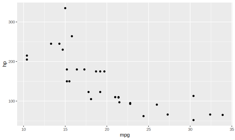
ggplot(mtcars, aes(x = mpg, y = hp)) + geom_point()

# Step 4: Test caTools: split the iris data 70 : 30
library(caTools)
set.seed(123)
split <- sample.split(iris$Species, SplitRatio = 0.7)
table(split)

# Step 5: Test rpart: a classification tree
library(rpart)
fit <- rpart(Species ~ ., data = iris)
fit

5. Execution and Results

Step 1: Install the packages

OUTPUT (typical; not run here)

Installing package into ...
...
* DONE (ggplot2)

Each command prints the download and ends with DONE.

Step 2: Check that they are installed

OUTPUT

[1] TRUE TRUE TRUE

Step 3: Test ggplot2: a scatter plot

PLOT

Practical 2: Test ggplot2: a scatter plot, as drawn by the R code above

Step 4: Test caTools: split the iris data 70 : 30

OUTPUT

split
FALSE  TRUE 
   45   105

Step 5: Test rpart: a classification tree

OUTPUT

n= 150 

node), split, n, loss, yval, (yprob)
      * denotes terminal node

1) root 150 100 setosa (0.33333333 0.33333333 0.33333333)  
  2) Petal.Length< 2.45 50   0 setosa (1.00000000 0.00000000 0.00000000) *
  3) Petal.Length>=2.45 100  50 versicolor (0.00000000 0.50000000 0.50000000)  
    6) Petal.Width< 1.75 54   5 versicolor (0.00000000 0.90740741 0.09259259) *
    7) Petal.Width>=1.75 46   1 virginica (0.00000000 0.02173913 0.97826087) *

Note. There is no package called "CART" on CRAN, so install.packages("CART") fails. Classification and regression trees in R come from rpart, which is installed with R.

Note. To install dependencies, dependencies = TRUE is an argument: install.packages("ggplot2", dependencies = TRUE), not a package name in quotes.

RESULT

The three packages are installed, and each works: ggplot2 draws, caTools splits 150 iris rows into 105 for training and 45 for testing, and rpart grows a tree.

Practical 3: Loading the Packages "ggplot2" and "caTools"

1. Question

Load the packages ggplot2 and caTools, confirm they are loaded, and use each once.

2. Aim

To load installed packages into the R session and confirm that they are attached.

3. Steps

Load the packages.
Confirm they are attached.
Use caTools: split mtcars into training and test sets.
Use ggplot2: the training set.

R COMMANDS AND FORMULAS USED

Command or formula	What it does
`library(name)`	loads the package; stops with an error if it is not installed
`(.packages())`	the packages attached in this session
`sample.split(y, SplitRatio)`	TRUE for rows chosen for training
`subset(data, condition)`	the rows that satisfy a condition

4. Programme

PRACTICAL 3 — THE R PROGRAMME

# Practical 3: Loading the Packages "ggplot2" and "caTools"

# Step 1: Load the packages
library(ggplot2)
library(caTools)

# Step 2: Confirm they are attached
c("ggplot2", "caTools") %in% (.packages())

# Step 3: Use caTools: split mtcars into training and test sets
set.seed(123)
split <- sample.split(mtcars$mpg, SplitRatio = 0.7)
train_set <- subset(mtcars, split == TRUE)
test_set  <- subset(mtcars, split == FALSE)
c(train = nrow(train_set), test = nrow(test_set))

# Step 4: Use ggplot2: the training set
ggplot(train_set, aes(x = wt, y = mpg)) + geom_point() +
  labs(title = "mtcars training set", x = "Weight (1000 lb)", y = "Miles per gallon")

5. Execution and Results

Step 1: Load the packages

Nothing is printed: this step only creates objects or loads packages.

Step 2: Confirm they are attached

OUTPUT

[1] TRUE TRUE

Step 3: Use caTools: split mtcars into training and test sets

OUTPUT

train  test 
   22    10

Step 4: Use ggplot2: the training set

PLOT

Practical 3: Use ggplot2: the training set, as drawn by the R code above

RESULT

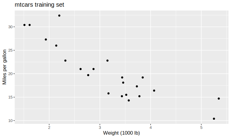
Both packages load without error and are attached. install.packages() is run once on a computer; library() is run in every new session.

Practical 4: Basic Operations in R

1. Question

Carry out the basic operations of R with examples: arithmetic, assignment, logical operations, vectors, matrices, statistical functions, sequences, conditions, loops and functions.

2. Aim

To learn the basic operations of R through small numerical examples.

3. Steps

Arithmetic.
Assignment.
Logical operations.
Vector operations.
Matrix operations.
+ adds element by element; %*% is the matrix product.
Statistical functions.
Sequences and repetition.
Conditional statements.
Loops.
Functions.

R COMMANDS AND FORMULAS USED

Command or formula	What it does
`+ - * / ^`	add, subtract, multiply, divide, power
`%%` and `%/%`	remainder and integer division
`<-` or `=`	assignment
`> < == != >= <=`, `& \| !`	comparisons, and logical and, or, not
`c()`, `matrix()`, `%*%`	vectors, matrices, matrix product
`mean() median() sd() var() summary()`	statistics
`seq() rep()`	sequences and repetition
`if / else`, `for`, `while`, `function`	control and functions

4. Programme

PRACTICAL 4 — THE R PROGRAMME

# Practical 4: Basic Operations in R

# Step 1: Arithmetic
5 + 3
10 - 4
6 * 7
20 / 4
2 ^ 3
10 %% 3
10 %/% 3

# Step 2: Assignment
a <- 15
b = 4
sum_result <- a + b
prod_result <- a * b
print(sum_result)
print(prod_result)

# Step 3: Logical operations
x <- 10
y <- 20
x > y
x < y
x == y
x != y
x >= y
(x > 5) & (y < 30)
(x > 5) | (y > 30)
!(x > y)

# Step 4: Vector operations
vec1 <- c(2, 4, 6)
vec2 <- c(1, 3, 5)
vec1 + vec2
vec1 * vec2
vec1 / vec2
vec1 > vec2

# Step 5: Matrix operations
mat1 <- matrix(c(1, 2, 3, 4), nrow = 2, ncol = 2)
mat2 <- matrix(c(5, 6, 7, 8), nrow = 2, ncol = 2)
mat1 + mat2
mat1 %*% mat2

# Step 6: Statistical functions
nums <- c(10, 20, 30, 40, 50)
mean(nums)
median(nums)
sd(nums)
var(nums)
min(nums)
max(nums)
summary(nums)

# Step 7: Sequences and repetition
seq(1, 10)
seq(1, 10, by = 2)
rep(5, times = 4)
rep(c(1, 2, 3), times = 3)

# Step 8: Conditional statements
x <- 15
if (x > 10) {
  print("x is greater than 10")
} else if (x == 10) {
  print("x is exactly 10")
} else {
  print("x is less than 10")
}

# Step 9: Loops
for (i in 1:5) {
  print(i)
}
x <- 1
while (x <= 3) {
  print(x)
  x <- x + 1
}

# Step 10: Functions
square <- function(num) {
  return(num ^ 2)
}
square(4)
square(5)

5. Execution and Results

Step 1: Arithmetic

OUTPUT

[1] 8
[1] 6
[1] 42
[1] 5
[1] 8
[1] 1
[1] 3

Step 2: Assignment

OUTPUT

[1] 19
[1] 60

Step 3: Logical operations

OUTPUT

[1] FALSE
[1] TRUE
[1] FALSE
[1] TRUE
[1] FALSE
[1] TRUE
[1] TRUE
[1] TRUE

Step 4: Vector operations

OUTPUT

[1]  3  7 11
[1]  2 12 30
[1] 2.000000 1.333333 1.200000
[1] TRUE TRUE TRUE

Step 5: Matrix operations

OUTPUT

     [,1] [,2]
[1,]    6   10
[2,]    8   12
     [,1] [,2]
[1,]   23   31
[2,]   34   46

Step 6: Statistical functions

OUTPUT

[1] 30
[1] 30
[1] 15.81139
[1] 250
[1] 10
[1] 50
   Min. 1st Qu.  Median    Mean 3rd Qu.    Max. 
     10      20      30      30      40      50

Step 7: Sequences and repetition

OUTPUT

 [1]  1  2  3  4  5  6  7  8  9 10
[1] 1 3 5 7 9
[1] 5 5 5 5
[1] 1 2 3 1 2 3 1 2 3

Step 8: Conditional statements

OUTPUT

[1] "x is greater than 10"

Step 9: Loops

OUTPUT

[1] 1
[1] 2
[1] 3
[1] 4
[1] 5
[1] 1
[1] 2
[1] 3

Step 10: Functions

OUTPUT

[1] 16
[1] 25

Note. sd() and var() divide by n − 1, the sample formulas: for 10, 20, 30, 40, 50 they give 15.81 and 250. Dividing by n would give 14.14 and 200.

RESULT

R works as a calculator, stores values in variables, compares them, and operates on whole vectors and matrices at once; its statistical functions, sequences, conditions, loops and user-written functions are the building blocks of every later practical.

Practical 5: Working with Vectors using R

1. Question

(a) Create a vector v1 with elements 1 to 20. (b) Add 2 to every element of v1. (c) Divide every element of v1 by 5. (d) Create a vector v2 with elements 21 to 30, and add v1 to v2.

2. Aim

To create vectors and operate on every element at once, and to see how R adds vectors of different lengths.

3. Steps

(a) Create v1 with elements 1 to 20.
(b) Add 2 to every element.
(c) Divide every element by 5.
(d) Create v2 with elements 21 to 30.
(d) Add v1 to v2.
v1 has 20 elements and v2 has 10. R recycles the shorter vector: v2 is used twice, so element 11 of v1 is added to element 1 of v2 again. Because 20 is a multiple of 10, R gives no warning.
When the lengths do not fit.
If the longer length is not a multiple of the shorter, R still recycles but warns.
Adding only the matching elements.
To add element by element without recycling, use the first ten elements of v1.

R COMMANDS AND FORMULAS USED

Command or formula	What it does
`a:b`	the whole numbers from a to b
`v + k`, `v / k`	applies the operation to every element
`v1 + v2`	adds element by element; a shorter vector is recycled
`v[1:10]`	the first ten elements
`length(v)`	the number of elements

4. Programme

PRACTICAL 5 — THE R PROGRAMME

# Practical 5: Working with Vectors using R

# Step 1: (a) Create v1 with elements 1 to 20
v1 <- 1:20
v1

# Step 2: (b) Add 2 to every element
v1 + 2

# Step 3: (c) Divide every element by 5
v1 / 5

# Step 4: (d) Create v2 with elements 21 to 30
v2 <- 21:30
v2
length(v1); length(v2)

# Step 5: (d) Add v1 to v2
v1 + v2

# Step 6: When the lengths do not fit
1:20 + 1:3

# Step 7: Adding only the matching elements
v1[1:10] + v2

5. Execution and Results

Step 1: (a) Create v1 with elements 1 to 20

OUTPUT

 [1]  1  2  3  4  5  6  7  8  9 10 11 12 13 14 15 16 17 18 19 20

Step 2: (b) Add 2 to every element

OUTPUT

 [1]  3  4  5  6  7  8  9 10 11 12 13 14 15 16 17 18 19 20 21 22

Step 3: (c) Divide every element by 5

OUTPUT

 [1] 0.2 0.4 0.6 0.8 1.0 1.2 1.4 1.6 1.8 2.0 2.2 2.4 2.6 2.8 3.0 3.2
[17] 3.4 3.6 3.8 4.0

Step 4: (d) Create v2 with elements 21 to 30

OUTPUT

 [1] 21 22 23 24 25 26 27 28 29 30
[1] 20
[1] 10

Step 5: (d) Add v1 to v2

OUTPUT

 [1] 22 24 26 28 30 32 34 36 38 40 32 34 36 38 40 42 44 46 48 50

Step 6: When the lengths do not fit

OUTPUT

 [1]  2  4  6  5  7  9  8 10 12 11 13 15 14 16 18 17 19 21 20 22
Warning message:
In 1:20 + 1:3 :
  longer object length is not a multiple of shorter object length

Step 7: Adding only the matching elements

OUTPUT

 [1] 22 24 26 28 30 32 34 36 38 40

Note. v1 + v2 with 20 and 10 elements gives no warning, because 20 is a multiple of 10; R recycles v2 silently. The warning "longer object length is not a multiple of shorter object length" appears only when it is not a multiple, as in 1:20 + 1:3.

RESULT

Arithmetic on a vector acts on every element. Adding two vectors works element by element, recycling the shorter one, which is why v1 + v2 has 20 elements: 22, 24, …, 40 and then 32, 34, …, 50.

Practical 6: Create the Matrix of the Data using R

1. Question

Using the distances between five cities in the table below, create a matrix M and find the pair of cities with the shortest distance.

	C1	C2	C3	C4	C5
C1	0	12	13	8	20
C2	12	0	15	28	88
C3	13	15	0	6	9
C4	8	28	6	0	33
C5	20	88	9	33	0

2. Aim

To store a table as a matrix with row and column names, and to search it for its smallest off-diagonal value.

3. Steps

Create the matrix M.
Check that the matrix is symmetric.
The distance from C1 to C2 must equal the distance from C2 to C1.
Find the shortest distance.
The diagonal (a city to itself) is 0 and must be left out, and each pair appears twice, above and below the diagonal. Looking only above the diagonal counts each pair once.
Name the pair of cities.

R COMMANDS AND FORMULAS USED

Command or formula	What it does
`matrix(x, nrow, ncol, byrow = TRUE)`	a matrix filled row by row
`rownames()`, `colnames()`	name the rows and columns
`upper.tri(M)`	TRUE above the diagonal: each pair of cities once
`min()`, `which(..., arr.ind = TRUE)`	the smallest value, and its row and column

4. Programme

PRACTICAL 6 — THE R PROGRAMME

# Practical 6: Create the Matrix of the Data using R

# Step 1: Create the matrix M
M <- matrix(c( 0, 12, 13,  8, 20,
              12,  0, 15, 28, 88,
              13, 15,  0,  6,  9,
               8, 28,  6,  0, 33,
              20, 88,  9, 33,  0),
            nrow = 5, ncol = 5, byrow = TRUE)
city <- c("C1", "C2", "C3", "C4", "C5")
rownames(M) <- city
colnames(M) <- city
M

# Step 2: Check that the matrix is symmetric
isSymmetric(M)

# Step 3: Find the shortest distance
pairs <- M[upper.tri(M)]
min_distance <- min(pairs)
min_distance

# Step 4: Name the pair of cities
where <- which(M == min_distance & upper.tri(M), arr.ind = TRUE)
where
cat("The shortest distance is", min_distance, "between",
    rownames(M)[where[1, "row"]], "and", colnames(M)[where[1, "col"]], "\n")

5. Execution and Results

Step 1: Create the matrix M

OUTPUT

   C1 C2 C3 C4 C5
C1  0 12 13  8 20
C2 12  0 15 28 88
C3 13 15  0  6  9
C4  8 28  6  0 33
C5 20 88  9 33  0

Step 2: Check that the matrix is symmetric

OUTPUT

[1] TRUE

Step 3: Find the shortest distance

OUTPUT

[1] 6

Step 4: Name the pair of cities

OUTPUT

   row col
C3   3   4
The shortest distance is 6 between C3 and C4

Note. Searching the whole matrix, as in which(M == min_distance, arr.ind = TRUE) after setting the zeros to Inf, returns two rows, (C4, C3) and (C3, C4), because the matrix is symmetric; its first row names the pair as "C4 and C3". Restricting the search to upper.tri(M) gives each pair once.

RESULT

The shortest distance is 6, between cities C3 and C4.

Practical 7: Create the Data Structures of the Data using R

1. Question

The marks scored by six students in two sections are:

Section	Student	M1	M2	M3
A	1	46	54	45
A	2	34	55	55
A	3	56	66	64
B	1	43	44	45
B	2	67	76	78
B	3	76	68	37

(a) Create a data structure for the data, with proper names. (b) Display the marks and totals of all students. (c) Display the highest total in each section. (d) Add a new subject, M4, with marks for both sections (50, 48, 67 for Section A and 54, 73, 42 for Section B).

2. Aim

To store mixed data in a data frame, add computed and new columns, and summarise by group.

3. Steps

(a) Create the data frame.
(b) Marks and totals of all students.
(c) The highest total in each section.
(d) Add a new subject M4 and recompute the totals.

R COMMANDS AND FORMULAS USED

Command or formula	What it does
`data.frame()`	a table whose columns may be of different types
`df$col`	one column; assigning to a new name adds a column
`rowSums(df[ , cols])`	the total of each row
`tapply(x, group, max)`	the maximum of x within each group

4. Programme

PRACTICAL 7 — THE R PROGRAMME

# Practical 7: Create the Data Structures of the Data using R

# Step 1: (a) Create the data frame
marks <- data.frame(
  Section = c("A", "A", "A", "B", "B", "B"),
  Student = c(1, 2, 3, 1, 2, 3),
  M1 = c(46, 34, 56, 43, 67, 76),
  M2 = c(54, 55, 66, 44, 76, 68),
  M3 = c(45, 55, 64, 45, 78, 37)
)
marks
str(marks)

# Step 2: (b) Marks and totals of all students
marks$Total <- rowSums(marks[ , c("M1", "M2", "M3")])
marks

# Step 3: (c) The highest total in each section
tapply(marks$Total, marks$Section, max)
marks[marks$Total == ave(marks$Total, marks$Section, FUN = max), ]

# Step 4: (d) Add a new subject M4 and recompute the totals
marks$M4 <- c(50, 48, 67, 54, 73, 42)
marks$Total <- rowSums(marks[ , c("M1", "M2", "M3", "M4")])
marks
tapply(marks$Total, marks$Section, max)

5. Execution and Results

Step 1: (a) Create the data frame

OUTPUT

  Section Student M1 M2 M3
1       A       1 46 54 45
2       A       2 34 55 55
3       A       3 56 66 64
4       B       1 43 44 45
5       B       2 67 76 78
6       B       3 76 68 37
'data.frame':	6 obs. of  5 variables:
 $ Section: chr  "A" "A" "A" "B" ...
 $ Student: num  1 2 3 1 2 3
 $ M1     : num  46 34 56 43 67 76
 $ M2     : num  54 55 66 44 76 68
 $ M3     : num  45 55 64 45 78 37

Step 2: (b) Marks and totals of all students

OUTPUT

  Section Student M1 M2 M3 Total
1       A       1 46 54 45   145
2       A       2 34 55 55   144
3       A       3 56 66 64   186
4       B       1 43 44 45   132
5       B       2 67 76 78   221
6       B       3 76 68 37   181

Step 3: (c) The highest total in each section

OUTPUT

  A   B 
186 221 
  Section Student M1 M2 M3 Total
3       A       3 56 66 64   186
5       B       2 67 76 78   221

Step 4: (d) Add a new subject M4 and recompute the totals

OUTPUT

  Section Student M1 M2 M3 Total M4
1       A       1 46 54 45   195 50
2       A       2 34 55 55   192 48
3       A       3 56 66 64   253 67
4       B       1 43 44 45   186 54
5       B       2 67 76 78   294 73
6       B       3 76 68 37   223 42
  A   B 
253 294

RESULT

With three subjects, the highest totals are 186 in Section A (student 3) and 221 in Section B (student 2). With M4 added, they become 253 and 294, for the same two students.

Practical 8: Create the Matrix of the Data using R with Row and Column Names

1. Question

Three people, P1, P2 and P3, intend to buy rolls, buns, cakes and bread, in different amounts, from one of two shops, S1 and S2. The prices (in rupees) and the quantities wanted are:

Item	Price at S1	Price at S2
Roll	1.5	1
Bun	2	2.5
Cake	5	4.5
Bread	16	17

Person	Roll	Bun	Cake	Bread
P1	6	5	3	1
P2	3	6	3	2
P3	3	4	3	1

(a) Create the matrices of this information with row and column names. (b) Display the demand and price matrices. (c) Find the total amount each person would spend in each shop. (d) Suggest the shop where each person should buy.

2. Aim

To represent the data as named matrices and use the matrix product to find each person's bill in each shop.

3. Steps

(a) Create the price matrix.
(a) Create the demand matrix.
(b) Display the two matrices.
(c) The total amount each person spends in each shop.
Each row of demand times each column of price is one bill. For P1 at S1: 6 × 1.5 + 5 × 2 + 3 × 5 + 1 × 16 = 9 + 10 + 15 + 16 = 50.
(d) The cheaper shop for each person.

R COMMANDS AND FORMULAS USED

Command or formula	What it does
`matrix(..., byrow = TRUE, dimnames = list(rows, cols))`	a named matrix
`D %*% P`	the matrix product: (3 × 4) times (4 × 2) gives 3 × 2
Total cost	person i at shop j = Σ_k quantity_ik × price_kj
`apply(m, 1, f)`	applies f to each row

4. Programme

PRACTICAL 8 — THE R PROGRAMME

# Practical 8: Create the Matrix of the Data using R with Row and Column Names

# Step 1: (a) Create the price matrix
price <- matrix(c(1.5, 1,
                  2,   2.5,
                  5,   4.5,
                  16,  17),
                nrow = 4, byrow = TRUE,
                dimnames = list(c("Roll", "Bun", "Cake", "Bread"), c("S1", "S2")))

# Step 2: (a) Create the demand matrix
demand <- matrix(c(6, 5, 3, 1,
                   3, 6, 3, 2,
                   3, 4, 3, 1),
                 nrow = 3, byrow = TRUE,
                 dimnames = list(c("P1", "P2", "P3"), c("Roll", "Bun", "Cake", "Bread")))

# Step 3: (b) Display the two matrices
price
demand

# Step 4: (c) The total amount each person spends in each shop
cost <- demand %*% price
cost

# Step 5: (d) The cheaper shop for each person
apply(cost, 1, function(r) if (r["S1"] < r["S2"]) "S1" else if (r["S1"] > r["S2"]) "S2" else "either")

5. Execution and Results

Step 1: (a) Create the price matrix

Nothing is printed: this step only creates objects or loads packages.

Step 2: (a) Create the demand matrix

Nothing is printed: this step only creates objects or loads packages.

Step 3: (b) Display the two matrices

OUTPUT

        S1   S2
Roll   1.5  1.0
Bun    2.0  2.5
Cake   5.0  4.5
Bread 16.0 17.0
   Roll Bun Cake Bread
P1    6   5    3     1
P2    3   6    3     2
P3    3   4    3     1

Step 4: (c) The total amount each person spends in each shop

OUTPUT

     S1   S2
P1 50.0 49.0
P2 63.5 65.5
P3 43.5 43.5

Step 5: (d) The cheaper shop for each person

OUTPUT

      P1       P2       P3 
    "S2"     "S1" "either"

Note. A commonly printed answer to this practical gives totals of 52.5 and 48.5 for P1, 59.0 and 60.0 for P2, and 52.5 and 50.5 for P3. Those are not the products of these two tables. Multiplying them out, as R does above, gives 50 and 49, 63.5 and 65.5, and 43.5 and 43.5.

RESULT

P1 spends ₹50 at S1 and ₹49 at S2, so should buy at S2; P2 spends ₹63.50 and ₹65.50, so should buy at S1; P3 spends ₹43.50 at either shop.

Practical 9: Applying the Summary of Data using R

1. Question

The marks in statistics of 50 candidates chosen at random from those appearing in an examination are:

32, 47, 41, 51, 41, 30, 39, 18, 48, 53, 54, 32, 31, 46, 15, 37, 32, 56, 42, 48, 38, 26, 50, 40, 38, 42, 35, 22, 62, 51, 44, 21, 45, 31, 37, 41, 44, 18, 37, 47, 68, 41, 30, 52, 52, 60, 42, 38, 38, 34

(a) Apply summary() to the data. (b) Calculate all the measures of dispersion. (c) Draw suitable graphs of the data.

2. Aim

To summarise a set of marks with R's built-in functions, measure their spread, and show their distribution in graphs.

3. Steps

Enter the data.
(a) Summary of the data.
The sorted marks show the order statistics behind the quartiles; table() gives the frequencies, from which the mode is read.
(b) Measures of dispersion.
(c) Histogram.
(c) Box plot.
(c) Density plot.

R COMMANDS AND FORMULAS USED

Command or formula	What it does
`summary(x)`	minimum, first quartile, median, mean, third quartile, maximum
Range	max − min: `diff(range(x))`
Variance	sample: Σ(x − x̄)² / (n − 1), `var(x)`; population: Σ(x − x̄)² / n
Standard deviation	the square root of the variance: `sd(x)` (sample)
Quartile deviation	(Q₃ − Q₁) / 2, with `IQR(x)` = Q₃ − Q₁
Mean deviation	Σ\|x − x̄\| / n
Coefficient of variation	s / x̄ × 100

4. Programme

PRACTICAL 9 — THE R PROGRAMME

# Practical 9: Applying the Summary of Data using R

# Step 1: Enter the data
marks <- c(32, 47, 41, 51, 41, 30, 39, 18, 48, 53,
           54, 32, 31, 46, 15, 37, 32, 56, 42, 48,
           38, 26, 50, 40, 38, 42, 35, 22, 62, 51,
           44, 21, 45, 31, 37, 41, 44, 18, 37, 47,
           68, 41, 30, 52, 52, 60, 42, 38, 38, 34)
length(marks)

# Step 2: (a) Summary of the data
summary(marks)
sort(marks)
freq <- table(marks)
names(freq)[freq == max(freq)]   # the mode(s)

# Step 3: (b) Measures of dispersion
n <- length(marks)
c(range = diff(range(marks)),
  variance_sample = var(marks),
  variance_population = var(marks) * (n - 1) / n,
  sd_sample = sd(marks),
  sd_population = sqrt(var(marks) * (n - 1) / n),
  IQR = IQR(marks),
  quartile_deviation = IQR(marks) / 2,
  mean_deviation = mean(abs(marks - mean(marks))),
  CV_percent = sd(marks) / mean(marks) * 100)

# Step 4: (c) Histogram
library(ggplot2)
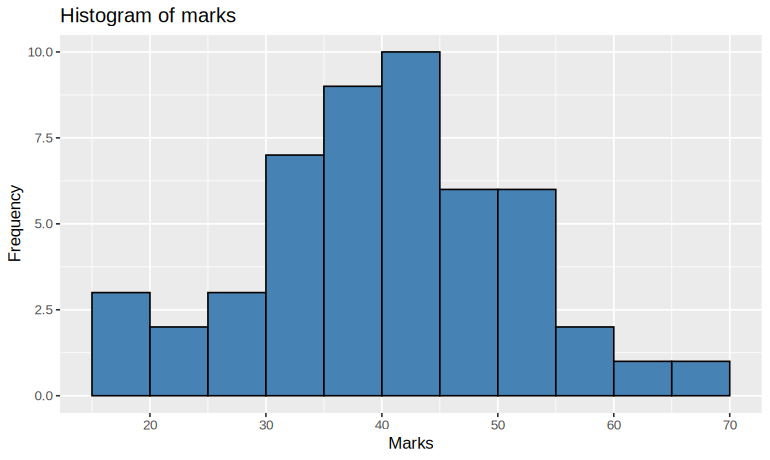
ggplot(data.frame(marks), aes(x = marks)) +
  geom_histogram(binwidth = 5, boundary = 15, fill = "steelblue", colour = "black") +
  labs(title = "Histogram of marks", x = "Marks", y = "Frequency")

# Step 5: (c) Box plot
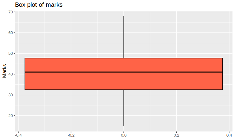
ggplot(data.frame(marks), aes(y = marks)) +
  geom_boxplot(fill = "tomato", colour = "black") +
  labs(title = "Box plot of marks", y = "Marks")

# Step 6: (c) Density plot
ggplot(data.frame(marks), aes(x = marks)) +
  geom_density(fill = "seagreen", alpha = 0.5) +
  labs(title = "Density of marks", x = "Marks", y = "Density")

5. Execution and Results

Step 1: Enter the data

OUTPUT

[1] 50

Step 2: (a) Summary of the data

OUTPUT

   Min. 1st Qu.  Median    Mean 3rd Qu.    Max. 
  15.00   32.50   41.00   40.34   47.75   68.00 
 [1] 15 18 18 21 22 26 30 30 31 31 32 32 32 34 35 37 37 37 38 38 38 38
[23] 39 40 41 41 41 41 42 42 42 44 44 45 46 47 47 48 48 50 51 51 52 52
[45] 53 54 56 60 62 68
[1] "38" "41"

Step 3: (b) Measures of dispersion

OUTPUT

              range     variance_sample variance_population 
           53.00000           130.22898           127.62440 
          sd_sample       sd_population                 IQR 
           11.41179            11.29710            15.25000 
 quartile_deviation      mean_deviation          CV_percent 
            7.62500             8.76640            28.28902

Step 4: (c) Histogram

PLOT

Practical 9: (c) Histogram, as drawn by the R code above

Step 5: (c) Box plot

PLOT

Practical 9: (c) Box plot, as drawn by the R code above

Step 6: (c) Density plot

PLOT

Practical 9: (c) Density plot, as drawn by the R code above

Note. Two values, 38 and 41, each occur four times, so the marks have two modes, not one.

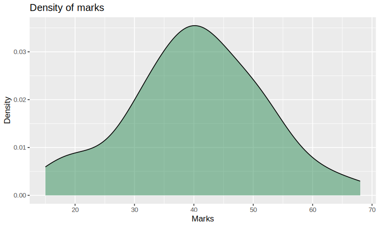
Note. R's var() and sd() divide by n − 1 and give 130.23 and 11.41. Dividing by n gives 127.62 and 11.30, the population figures that are often printed; the coefficient of variation is then 28.0% instead of 28.3%. State which divisor you use.

Note. In R, mad() is the median absolute deviation (scaled by 1.4826), not the mean deviation; the mean deviation about the mean is mean(abs(x - mean(x))) = 8.77.

RESULT

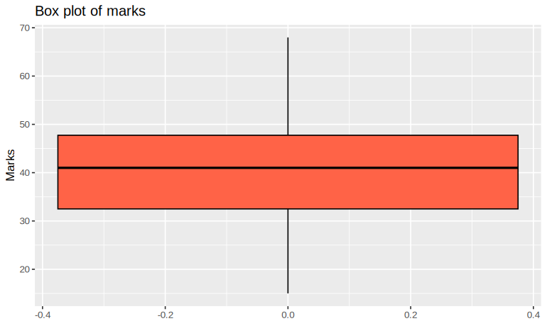
The marks run from 15 to 68 (range 53), with mean 40.34, median 41 and modes 38 and 41. The quartiles are 32.5 and 47.75, so the IQR is 15.25. The sample standard deviation is 11.41 and the coefficient of variation 28.3%. The histogram and density plot show one central peak around 40, slightly longer on the left; the box plot shows no outliers.

Practical 10: Implementation of Data Visualizations using R

1. Question

(i) For the 50 marks of Practical 9, draw a histogram, a box plot and a line plot.

(ii) Draw a bar chart of the chlorophyll data, and a multiple bar chart of the production data.

Chlorophyll type	Frequency
Albina	50
Xantha	44
Chloria	36
Viridis	30
Xchloro-viridis	16
Chlorotica	16
Virescent	8

Year	Wheat	Maize	Rice
1984	0.51	0.52	1.38
1985	0.51	1.38	2.02
1986	0.65	1.41	1.91
1987	0.36	1.64	2.26

(iii) Draw a scatter plot of marks1 (the marks of Practical 9) against marks2:

30, 42, 41, 31, 41, 38, 39, 18, 28, 53, 64, 32, 41, 26, 25, 37, 32, 56, 52, 18, 48, 76, 20, 10, 48, 45, 39, 29, 69, 52, 47, 28, 47, 32, 67, 51, 44, 19, 27, 42, 66, 21, 60, 22, 52, 64, 49, 33, 35, 37

2. Aim

To draw the standard graphs of R, each suited to a different kind of data: bar, multiple bar, histogram, box, line and scatter plots.

3. Steps

The data.
(ii) Bar chart of the chlorophyll types.
factor(..., levels = ...) keeps the bars in the table's order, not alphabetical.
(ii) Multiple bar chart of crop production.
(i) Histogram of the marks.
(i) Box plot of the marks.
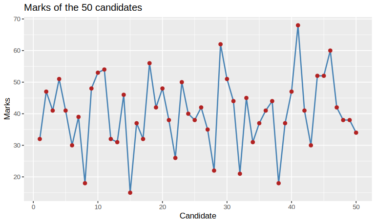
(i) Line plot of the marks, in the order given.
(iii) Scatter plot of marks1 against marks2.
The two vectors go into one data frame first, so that ggplot() plots these marks and not another data set.

R COMMANDS AND FORMULAS USED

Command or formula	What it does
Bar chart	`geom_col()` (or `geom_bar(stat = "identity")`): categories against their frequencies
Multiple bar chart	`geom_col(position = "dodge")`: one bar per group within each category
Histogram	`geom_histogram()`: the distribution of a continuous variable
Box plot	`geom_boxplot()`: median, quartiles and outliers
Line plot	`geom_line()`: values in order
Scatter plot	`geom_point()`: one variable against another; `cor()` measures the linear relation

4. Programme

PRACTICAL 10 — THE R PROGRAMME

# Practical 10: Implementation of Data Visualizations using R

# Step 1: The data
library(ggplot2)
marks1 <- c(32, 47, 41, 51, 41, 30, 39, 18, 48, 53,
            54, 32, 31, 46, 15, 37, 32, 56, 42, 48,
            38, 26, 50, 40, 38, 42, 35, 22, 62, 51,
            44, 21, 45, 31, 37, 41, 44, 18, 37, 47,
            68, 41, 30, 52, 52, 60, 42, 38, 38, 34)
marks2 <- c(30, 42, 41, 31, 41, 38, 39, 18, 28, 53,
            64, 32, 41, 26, 25, 37, 32, 56, 52, 18,
            48, 76, 20, 10, 48, 45, 39, 29, 69, 52,
            47, 28, 47, 32, 67, 51, 44, 19, 27, 42,
            66, 21, 60, 22, 52, 64, 49, 33, 35, 37)
chlorophyll <- data.frame(
  Type = c("Albina", "Xantha", "Chloria", "Viridis", "Xchloro-viridis", "Chlorotica", "Virescent"),
  Frequency = c(50, 44, 36, 30, 16, 16, 8))
crops <- data.frame(
  Year = rep(c(1984, 1985, 1986, 1987), each = 3),
  Crop = rep(c("Wheat", "Maize", "Rice"), times = 4),
  Production = c(0.51, 0.52, 1.38, 0.51, 1.38, 2.02, 0.65, 1.41, 1.91, 0.36, 1.64, 2.26))
c(length(marks1), length(marks2))

# Step 2: (ii) Bar chart of the chlorophyll types
chlorophyll$Type <- factor(chlorophyll$Type, levels = chlorophyll$Type)
ggplot(chlorophyll, aes(x = Type, y = Frequency)) +
  geom_col(fill = "skyblue", colour = "black") +
  labs(title = "Chlorophyll types", x = "Type", y = "Frequency")

# Step 3: (ii) Multiple bar chart of crop production
ggplot(crops, aes(x = factor(Year), y = Production, fill = Crop)) +
  geom_col(position = "dodge", colour = "black") +
  labs(title = "Production of wheat, maize and rice", x = "Year", y = "Production")

# Step 4: (i) Histogram of the marks
ggplot(data.frame(marks1), aes(x = marks1)) +
  geom_histogram(binwidth = 5, boundary = 15, fill = "steelblue", colour = "black") +
  labs(title = "Histogram of marks", x = "Marks", y = "Frequency")

# Step 5: (i) Box plot of the marks
ggplot(data.frame(marks1), aes(y = marks1)) +
  geom_boxplot(fill = "tomato", colour = "black") +
  labs(title = "Box plot of marks", y = "Marks")

# Step 6: (i) Line plot of the marks, in the order given
ggplot(data.frame(candidate = seq_along(marks1), marks1), aes(x = candidate, y = marks1)) +
  geom_line(colour = "steelblue", linewidth = 0.8) +
  geom_point(colour = "firebrick", size = 2) +
  labs(title = "Marks of the 50 candidates", x = "Candidate", y = "Marks")

# Step 7: (iii) Scatter plot of marks1 against marks2
pairs <- data.frame(marks1, marks2)
ggplot(pairs, aes(x = marks1, y = marks2)) +
  geom_point(colour = "steelblue", size = 2.5) +
  labs(title = "marks1 against marks2", x = "marks1", y = "marks2")
round(cor(marks1, marks2), 3)

5. Execution and Results

Step 1: The data

OUTPUT

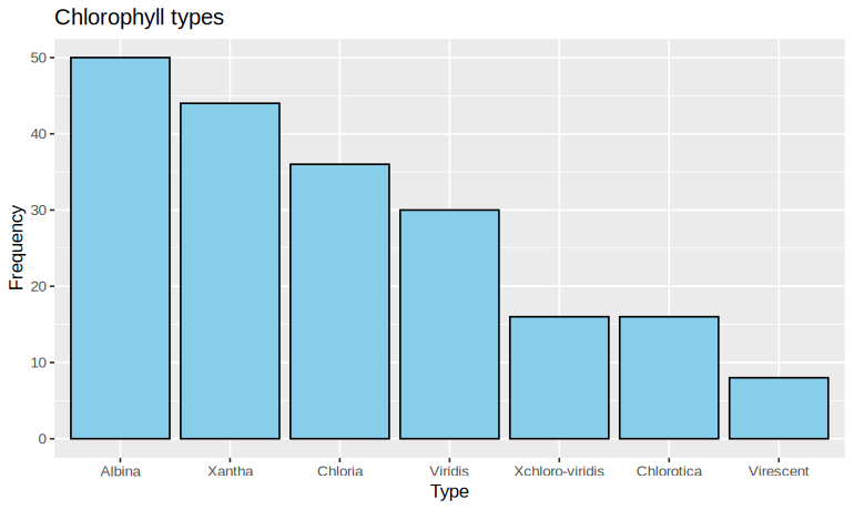
[1] 50 50

Step 2: (ii) Bar chart of the chlorophyll types

PLOT

Practical 10: (ii) Bar chart of the chlorophyll types, as drawn by the R code above

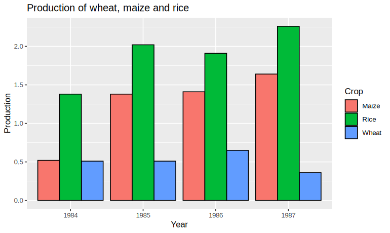
Step 3: (ii) Multiple bar chart of crop production

PLOT

Practical 10: (ii) Multiple bar chart of crop production, as drawn by the R code above

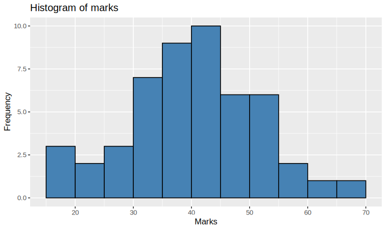
Step 4: (i) Histogram of the marks

PLOT

Practical 10: (i) Histogram of the marks, as drawn by the R code above

Step 5: (i) Box plot of the marks

PLOT

Practical 10: (i) Box plot of the marks, as drawn by the R code above

Step 6: (i) Line plot of the marks, in the order given

PLOT

Practical 10: (i) Line plot of the marks, in the order given, as drawn by the R code above

Step 7: (iii) Scatter plot of marks1 against marks2

OUTPUT

[1] 0.409

PLOT

Practical 10: (iii) Scatter plot of marks1 against marks2, as drawn by the R code above

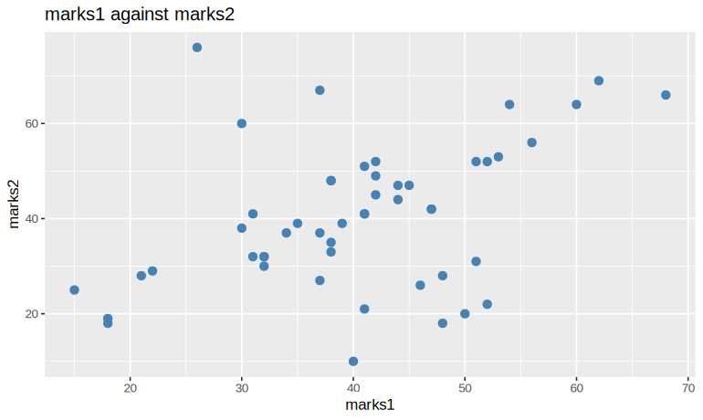
Note. For the scatter plot, marks1 and marks2 must be put into a data frame (pairs <- data.frame(marks1, marks2)) before ggplot(). A version with that line commented out plots whatever data frame was last called data.

Note. In ggplot2 3.4 and later, the thickness of a line is set with linewidth; size still works for points but is deprecated for lines.

RESULT

The bar chart compares the seven chlorophyll types, with Albina the most frequent; the multiple bar chart shows rice the largest crop in every year. The histogram, box plot and line plot show the marks' distribution and their variation from candidate to candidate; the scatter plot shows marks2 tending to rise with marks1, a moderate positive relation (correlation 0.41).

← Previous: Unit 5 Next: Syllabus →

Practical Course — 10 Practicals

The syllabus exercises and the practicals

Practical 1: Installing R and RStudio

1. Question

2. Aim

3. Steps

4. Programme

5. Execution and Results

Step 3: Check the installation

Step 4: Create the folder DS_R and make it the working directory

Practical 2: Installing the Packages "ggplot2", "caTools" and "CART"

1. Question

2. Aim

3. Steps

4. Programme

5. Execution and Results

Step 1: Install the packages

Step 2: Check that they are installed

Step 3: Test ggplot2: a scatter plot

Step 4: Test caTools: split the iris data 70 : 30

Step 5: Test rpart: a classification tree

Practical 3: Loading the Packages "ggplot2" and "caTools"

1. Question

2. Aim

3. Steps

4. Programme

5. Execution and Results

Step 1: Load the packages

Step 2: Confirm they are attached

Step 3: Use caTools: split mtcars into training and test sets

Step 4: Use ggplot2: the training set

Practical 4: Basic Operations in R

1. Question

2. Aim

3. Steps

4. Programme

5. Execution and Results

Step 1: Arithmetic

Step 2: Assignment

Step 3: Logical operations

Step 4: Vector operations

Step 5: Matrix operations

Step 6: Statistical functions

Step 7: Sequences and repetition

Step 8: Conditional statements

Step 9: Loops

Step 10: Functions

Practical 5: Working with Vectors using R

1. Question

2. Aim

3. Steps

4. Programme

5. Execution and Results

Step 1: (a) Create v1 with elements 1 to 20

Step 2: (b) Add 2 to every element

Step 3: (c) Divide every element by 5

Step 4: (d) Create v2 with elements 21 to 30

Step 5: (d) Add v1 to v2

Step 6: When the lengths do not fit

Step 7: Adding only the matching elements

Practical 6: Create the Matrix of the Data using R

1. Question

2. Aim

3. Steps

4. Programme

5. Execution and Results

Step 1: Create the matrix M

Step 2: Check that the matrix is symmetric

Step 3: Find the shortest distance

Step 4: Name the pair of cities

Practical 7: Create the Data Structures of the Data using R

1. Question

2. Aim

3. Steps

4. Programme

5. Execution and Results

Step 1: (a) Create the data frame

Step 2: (b) Marks and totals of all students

Step 3: (c) The highest total in each section

Step 4: (d) Add a new subject M4 and recompute the totals